Bayesian Supervised Learning in StochTree
Bayesian-Supervised-Learning.RmdThis vignette demonstrates how to use the bart()
function for supervised learning. To begin, we load the stochtree
package.
Demo 1: Step Function
Simulation
Here, we generate data from a simple step function.
# Generate the data
n <- 500
p_x <- 10
snr <- 3
X <- matrix(runif(n*p_x), ncol = p_x)
f_XW <- (
    ((0 <= X[,1]) & (0.25 > X[,1])) * (-7.5) +
    ((0.25 <= X[,1]) & (0.5 > X[,1])) * (-2.5) +
    ((0.5 <= X[,1]) & (0.75 > X[,1])) * (2.5) +
    ((0.75 <= X[,1]) & (1 > X[,1])) * (7.5)
)
noise_sd <- sd(f_XW) / snr
y <- f_XW + rnorm(n, 0, 1)*noise_sd

# Split data into test and train sets
test_set_pct <- 0.2
n_test <- round(test_set_pct*n)
n_train <- n - n_test
test_inds <- sort(sample(1:n, n_test, replace = F))
train_inds <- (1:n)[!((1:n) %in% test_inds)]
X_test <- X[test_inds,]
X_train <- X[train_inds,]
W_test <- NULL
W_train <- NULL
y_test <- y[test_inds]
y_train <- y[train_inds]
Sampling and Analysis
Warmstart
We first simulate from an ensemble model of \(y \mid X\) using “warm-start”
initialization samples (He and Hahn
(2023)). This is the default in stochtree.
num_gfr <- 10
num_burnin <- 0
num_mcmc <- 100
num_samples <- num_gfr + num_burnin + num_mcmc
bart_model_warmstart <- stochtree::bart(
    X_train = X_train, y_train = y_train, X_test = X_test, leaf_model = 0,
    num_trees = 100, num_gfr = num_gfr, num_burnin = num_burnin,
    num_mcmc = num_mcmc, sample_sigma = T, sample_tau = T
)
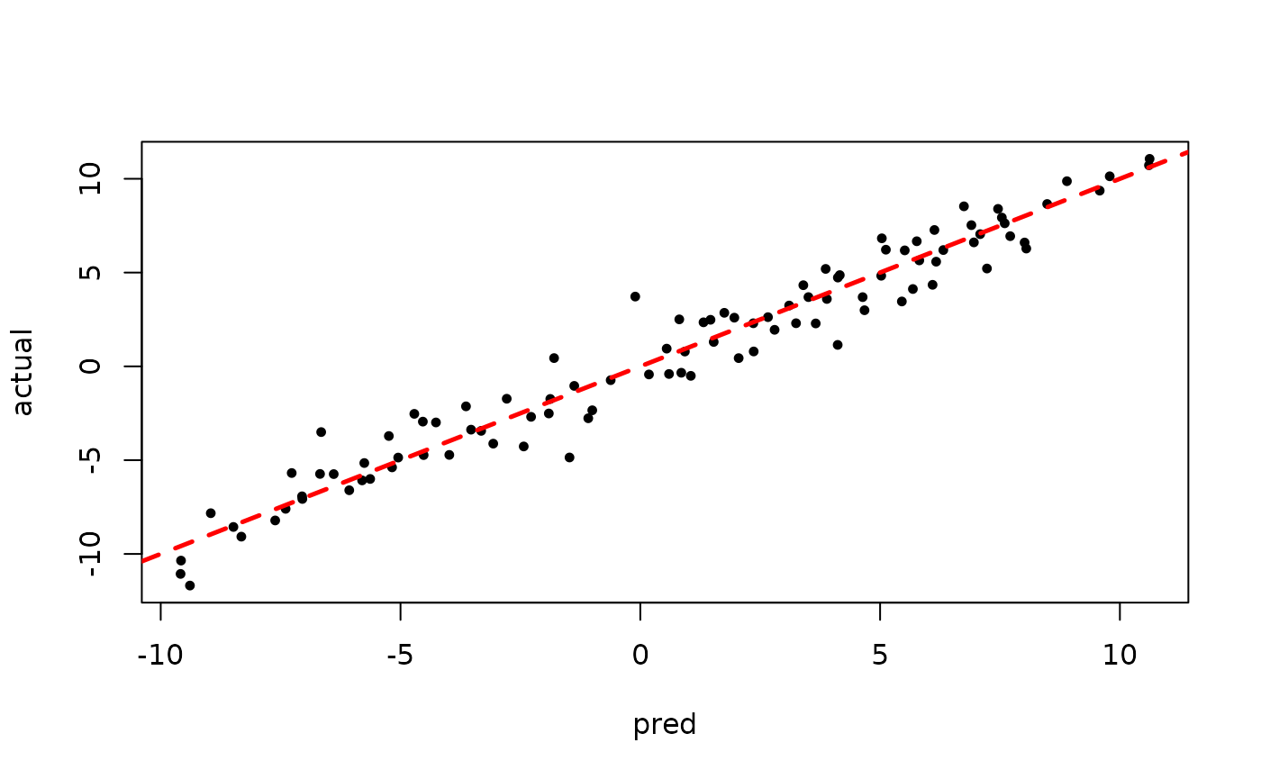
Inspect the initial XBART “warm-start” samples
plot(bart_model_warmstart$sigma2_samples[1:num_gfr], ylab="sigma^2")
plot(rowMeans(bart_model_warmstart$yhat_test[,1:num_gfr]), y_test, pch=16,
     cex=0.75, xlab = "pred", ylab = "actual")
abline(0,1,col="red",lty=2,lwd=2.5)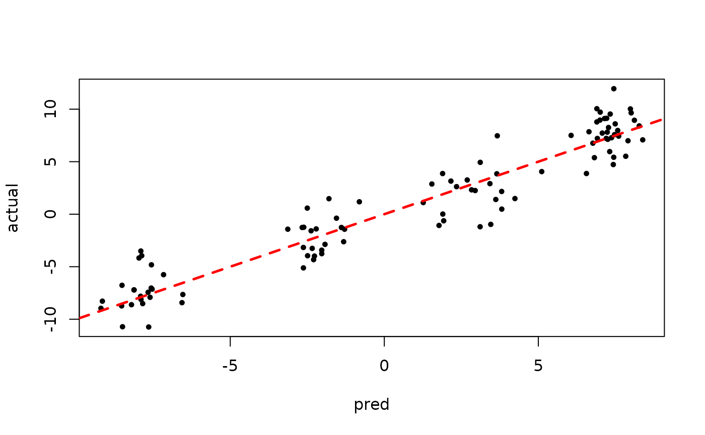
Inspect the BART samples that were initialized with an XBART warm-start
plot(bart_model_warmstart$sigma2_samples[(num_gfr + 1):num_samples], ylab="sigma^2")
plot(rowMeans(bart_model_warmstart$yhat_test[,(num_gfr + 1):num_samples]), y_test,
     pch=16, cex=0.75, xlab = "pred", ylab = "actual")
abline(0,1,col="red",lty=2,lwd=2.5)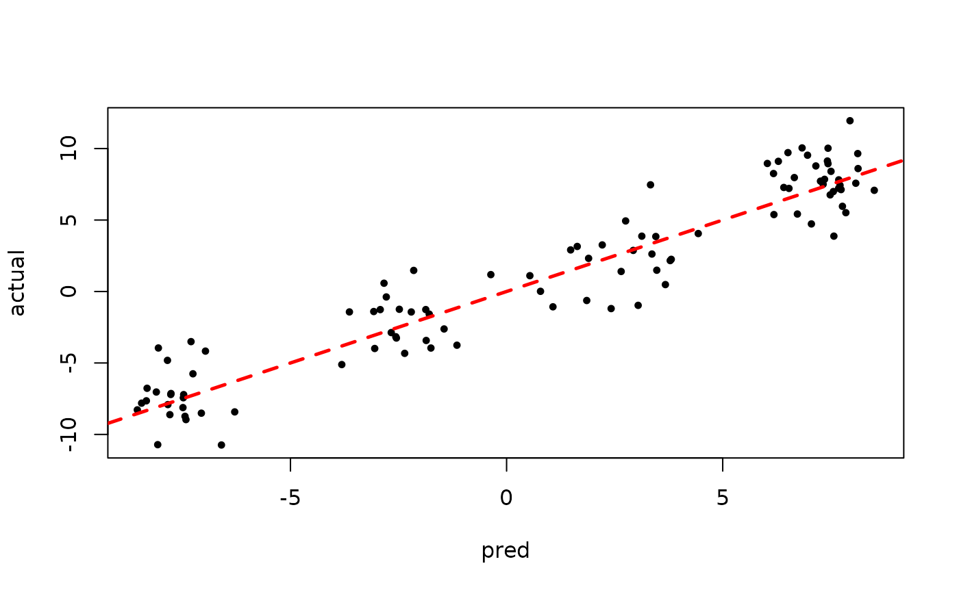
BART MCMC without Warmstart
Next, we simulate from this ensemble model without any warm-start initialization.
num_gfr <- 0
num_burnin <- 100
num_mcmc <- 100
num_samples <- num_gfr + num_burnin + num_mcmc
bart_model_root <- stochtree::bart(
    X_train = X_train, y_train = y_train, X_test = X_test, leaf_model = 0,
    num_trees = 100, num_gfr = num_gfr, num_burnin = num_burnin,
    num_mcmc = num_mcmc, sample_sigma = T, sample_tau = T
)
Inspect the BART samples after burnin.
plot(bart_model_root$sigma2_samples[(num_burnin + 1):num_samples], ylab="sigma^2")
plot(rowMeans(bart_model_root$yhat_test[,(num_burnin + 1):num_samples]), y_test,
     pch=16, cex=0.75, xlab = "pred", ylab = "actual")
abline(0,1,col="red",lty=2,lwd=2.5)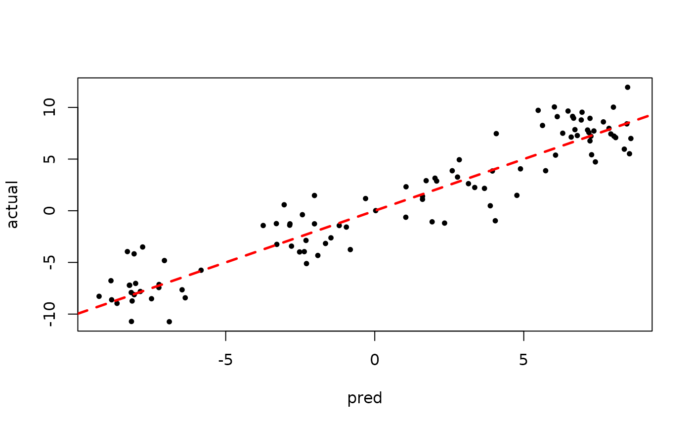
Demo 2: Partitioned Linear Model
Simulation
Here, we generate data from a simple partitioned linear model.
# Generate the data
n <- 500
p_x <- 10
p_w <- 1
snr <- 3
X <- matrix(runif(n*p_x), ncol = p_x)
W <- matrix(runif(n*p_w), ncol = p_w)
f_XW <- (
    ((0 <= X[,1]) & (0.25 > X[,1])) * (-7.5*W[,1]) +
    ((0.25 <= X[,1]) & (0.5 > X[,1])) * (-2.5*W[,1]) +
    ((0.5 <= X[,1]) & (0.75 > X[,1])) * (2.5*W[,1]) +
    ((0.75 <= X[,1]) & (1 > X[,1])) * (7.5*W[,1])
)
noise_sd <- sd(f_XW) / snr
y <- f_XW + rnorm(n, 0, 1)*noise_sd

# Split data into test and train sets
test_set_pct <- 0.2
n_test <- round(test_set_pct*n)
n_train <- n - n_test
test_inds <- sort(sample(1:n, n_test, replace = F))
train_inds <- (1:n)[!((1:n) %in% test_inds)]
X_test <- X[test_inds,]
X_train <- X[train_inds,]
W_test <- W[test_inds,]
W_train <- W[train_inds,]
y_test <- y[test_inds]
y_train <- y[train_inds]
Sampling and Analysis
Warmstart
We first simulate from an ensemble model of \(y \mid X\) using “warm-start”
initialization samples (He and Hahn
(2023)). This is the default in stochtree.
num_gfr <- 10
num_burnin <- 0
num_mcmc <- 100
num_samples <- num_gfr + num_burnin + num_mcmc
bart_model_warmstart <- stochtree::bart(
    X_train = X_train, W_train = W_train, y_train = y_train,
    X_test = X_test, W_test = W_test, leaf_model = 1,
    num_trees = 100, num_gfr = num_gfr, num_burnin = num_burnin,
    num_mcmc = num_mcmc, sample_sigma = T, sample_tau = T
)
Inspect the initial XBART “warm-start” samples
plot(bart_model_warmstart$sigma2_samples[1:num_gfr], ylab="sigma^2")
plot(rowMeans(bart_model_warmstart$yhat_test[,1:num_gfr]), y_test, pch=16,
     cex=0.75, xlab = "pred", ylab = "actual")
abline(0,1,col="red",lty=2,lwd=2.5)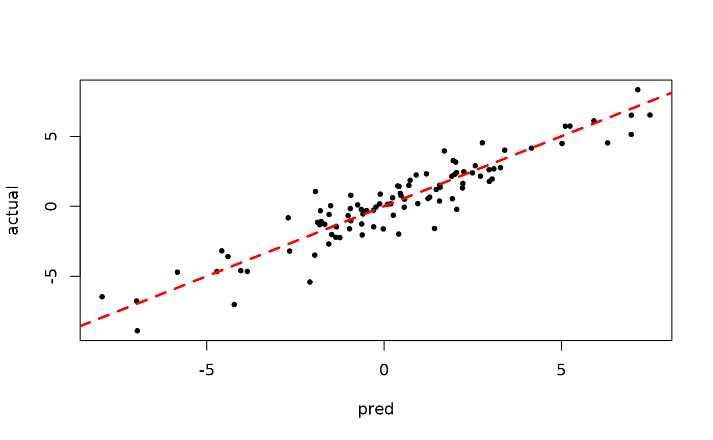
Inspect the BART samples that were initialized with an XBART warm-start
plot(bart_model_warmstart$sigma2_samples[(num_gfr + 1):num_samples], ylab="sigma^2")
plot(rowMeans(bart_model_warmstart$yhat_test[,(num_gfr + 1):num_samples]), y_test,
     pch=16, cex=0.75, xlab = "pred", ylab = "actual")
abline(0,1,col="red",lty=2,lwd=2.5)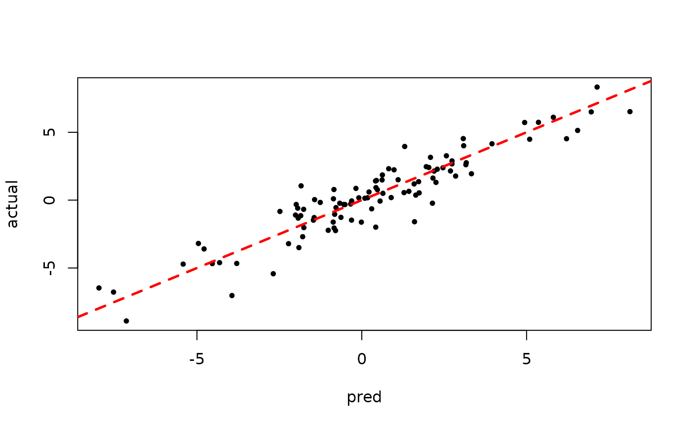
BART MCMC without Warmstart
Next, we simulate from this ensemble model without any warm-start initialization.
num_gfr <- 0
num_burnin <- 100
num_mcmc <- 100
num_samples <- num_gfr + num_burnin + num_mcmc
bart_model_root <- stochtree::bart(
    X_train = X_train, W_train = W_train, y_train = y_train,
    X_test = X_test, W_test = W_test, leaf_model = 1,
    num_trees = 100, num_gfr = num_gfr, num_burnin = num_burnin,
    num_mcmc = num_mcmc, sample_sigma = T, sample_tau = T
)
Inspect the BART samples after burnin.
plot(bart_model_root$sigma2_samples[(num_burnin + 1):num_samples], ylab="sigma^2")
plot(rowMeans(bart_model_root$yhat_test[,(num_burnin + 1):num_samples]), y_test,
     pch=16, cex=0.75, xlab = "pred", ylab = "actual")
abline(0,1,col="red",lty=2,lwd=2.5)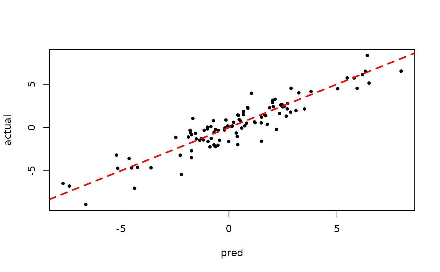
Demo 3: Partitioned Linear Model with Random Effects
Simulation
Here, we generate data from a simple partitioned linear model with an additive random effect structure.
# Generate the data
n <- 500
p_x <- 10
p_w <- 1
snr <- 3
X <- matrix(runif(n*p_x), ncol = p_x)
W <- matrix(runif(n*p_w), ncol = p_w)
group_ids <- rep(c(1,2), n %/% 2)
rfx_coefs <- matrix(c(-5, -3, 5, 3),nrow=2,byrow=T)
rfx_basis <- cbind(1, runif(n, -1, 1))
f_XW <- (
    ((0 <= X[,1]) & (0.25 > X[,1])) * (-7.5*W[,1]) +
    ((0.25 <= X[,1]) & (0.5 > X[,1])) * (-2.5*W[,1]) +
    ((0.5 <= X[,1]) & (0.75 > X[,1])) * (2.5*W[,1]) +
    ((0.75 <= X[,1]) & (1 > X[,1])) * (7.5*W[,1])
)
rfx_term <- rowSums(rfx_coefs[group_ids,] * rfx_basis)
noise_sd <- sd(f_XW) / snr
y <- f_XW + rfx_term + rnorm(n, 0, 1)*noise_sd

# Split data into test and train sets
test_set_pct <- 0.2
n_test <- round(test_set_pct*n)
n_train <- n - n_test
test_inds <- sort(sample(1:n, n_test, replace = F))
train_inds <- (1:n)[!((1:n) %in% test_inds)]
X_test <- X[test_inds,]
X_train <- X[train_inds,]
W_test <- W[test_inds,]
W_train <- W[train_inds,]
y_test <- y[test_inds]
y_train <- y[train_inds]
group_ids_test <- group_ids[test_inds]
group_ids_train <- group_ids[train_inds]
rfx_basis_test <- rfx_basis[test_inds,]
rfx_basis_train <- rfx_basis[train_inds,]
Sampling and Analysis
Warmstart
We first simulate from an ensemble model of \(y \mid X\) using “warm-start”
initialization samples (He and Hahn
(2023)). This is the default in stochtree.
num_gfr <- 10
num_burnin <- 0
num_mcmc <- 100
num_samples <- num_gfr + num_burnin + num_mcmc
bart_model_warmstart <- stochtree::bart(
    X_train = X_train, W_train = W_train, y_train = y_train,
    group_ids_train = group_ids_train, rfx_basis_train = rfx_basis_train,
    X_test = X_test, W_test = W_test, group_ids_test = group_ids_test,
    rfx_basis_test = rfx_basis_test, leaf_model = 1, num_trees = 100,
    num_gfr = num_gfr, num_burnin = num_burnin, num_mcmc = num_mcmc,
    sample_sigma = T, sample_tau = T
)
Inspect the initial XBART “warm-start” samples
plot(bart_model_warmstart$sigma2_samples[1:num_gfr], ylab="sigma^2")
abline(h=noise_sd^2,col="red",lty=2,lwd=2.5)
plot(rowMeans(bart_model_warmstart$yhat_test[,1:num_gfr]), y_test, pch=16,
     cex=0.75, xlab = "pred", ylab = "actual")
abline(0,1,col="red",lty=2,lwd=2.5)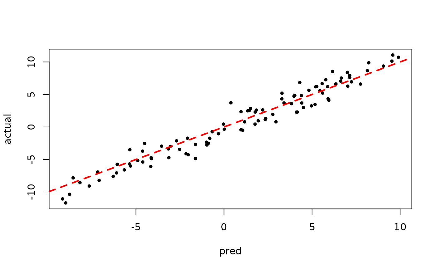
Inspect the BART samples that were initialized with an XBART warm-start
plot(bart_model_warmstart$sigma2_samples[(num_gfr + 1):num_samples], ylab="sigma^2")
abline(h=noise_sd^2,col="red",lty=2,lwd=2.5)
plot(rowMeans(bart_model_warmstart$yhat_test[,(num_gfr + 1):num_samples]), y_test,
     pch=16, cex=0.75, xlab = "pred", ylab = "actual")
abline(0,1,col="red",lty=2,lwd=2.5)
BART MCMC without Warmstart
Next, we simulate from this ensemble model without any warm-start initialization.
num_gfr <- 0
num_burnin <- 100
num_mcmc <- 100
num_samples <- num_gfr + num_burnin + num_mcmc
bart_model_root <- stochtree::bart(
    X_train = X_train, W_train = W_train, y_train = y_train,
    group_ids_train = group_ids_train, rfx_basis_train = rfx_basis_train,
    X_test = X_test, W_test = W_test, group_ids_test = group_ids_test,
    rfx_basis_test = rfx_basis_test, leaf_model = 1, num_trees = 100,
    num_gfr = num_gfr, num_burnin = num_burnin, num_mcmc = num_mcmc,
    sample_sigma = T, sample_tau = T
)
Inspect the BART samples after burnin.
plot(bart_model_root$sigma2_samples[(num_burnin + 1):num_samples], ylab="sigma^2")
abline(h=noise_sd^2,col="red",lty=2,lwd=2.5)
plot(rowMeans(bart_model_root$yhat_test[,(num_burnin + 1):num_samples]), y_test,
     pch=16, cex=0.75, xlab = "pred", ylab = "actual")
abline(0,1,col="red",lty=2,lwd=2.5)