Bayesian Supervised Learning in StochTree • stochtree

This vignette demonstrates how to use the bart() function for Bayesian supervised learning (Chipman, George, and McCulloch (2010)). To begin, we load the stochtree package.

library(stochtree)

Demo 1: Step Function

Simulation

Here, we generate data from a simple step function.

# Generate the data
n <- 500
p_x <- 10
snr <- 3
X <- matrix(runif(n*p_x), ncol = p_x)
f_XW <- (
    ((0 <= X[,1]) & (0.25 > X[,1])) * (-7.5) + 
    ((0.25 <= X[,1]) & (0.5 > X[,1])) * (-2.5) + 
    ((0.5 <= X[,1]) & (0.75 > X[,1])) * (2.5) + 
    ((0.75 <= X[,1]) & (1 > X[,1])) * (7.5)
)
noise_sd <- sd(f_XW) / snr
y <- f_XW + rnorm(n, 0, 1)*noise_sd

# Split data into test and train sets
test_set_pct <- 0.2
n_test <- round(test_set_pct*n)
n_train <- n - n_test
test_inds <- sort(sample(1:n, n_test, replace = FALSE))
train_inds <- (1:n)[!((1:n) %in% test_inds)]
X_test <- as.data.frame(X[test_inds,])
X_train <- as.data.frame(X[train_inds,])
W_test <- NULL
W_train <- NULL
y_test <- y[test_inds]
y_train <- y[train_inds]

Sampling and Analysis

Warmstart

We first sample from an ensemble model of $y \mid X$ using “warm-start” initialization samples (He and Hahn (2023)). This is the default in stochtree.

num_gfr <- 10
num_burnin <- 0
num_mcmc <- 100
num_samples <- num_gfr + num_burnin + num_mcmc
bart_model_warmstart <- stochtree::bart(
    X_train = X_train, y_train = y_train, X_test = X_test, 
    num_trees = 100, num_gfr = num_gfr, num_burnin = num_burnin, 
    num_mcmc = num_mcmc, sample_sigma = T, sample_tau = T
)

Inspect the MCMC samples

plot(bart_model_warmstart$sigma2_samples, ylab="sigma^2")

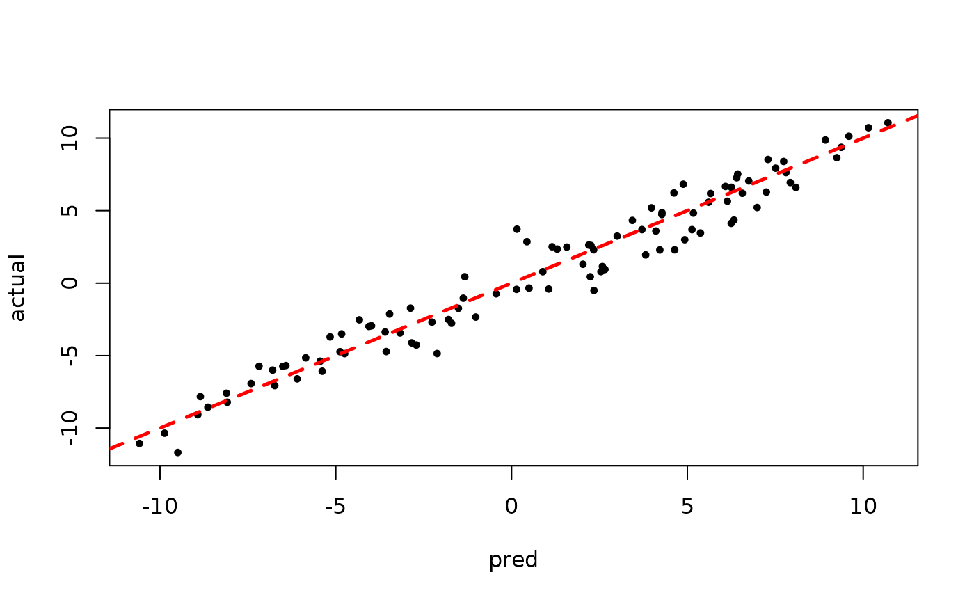
plot(rowMeans(bart_model_warmstart$y_hat_test), y_test, 
     pch=16, cex=0.75, xlab = "pred", ylab = "actual")
abline(0,1,col="red",lty=2,lwd=2.5)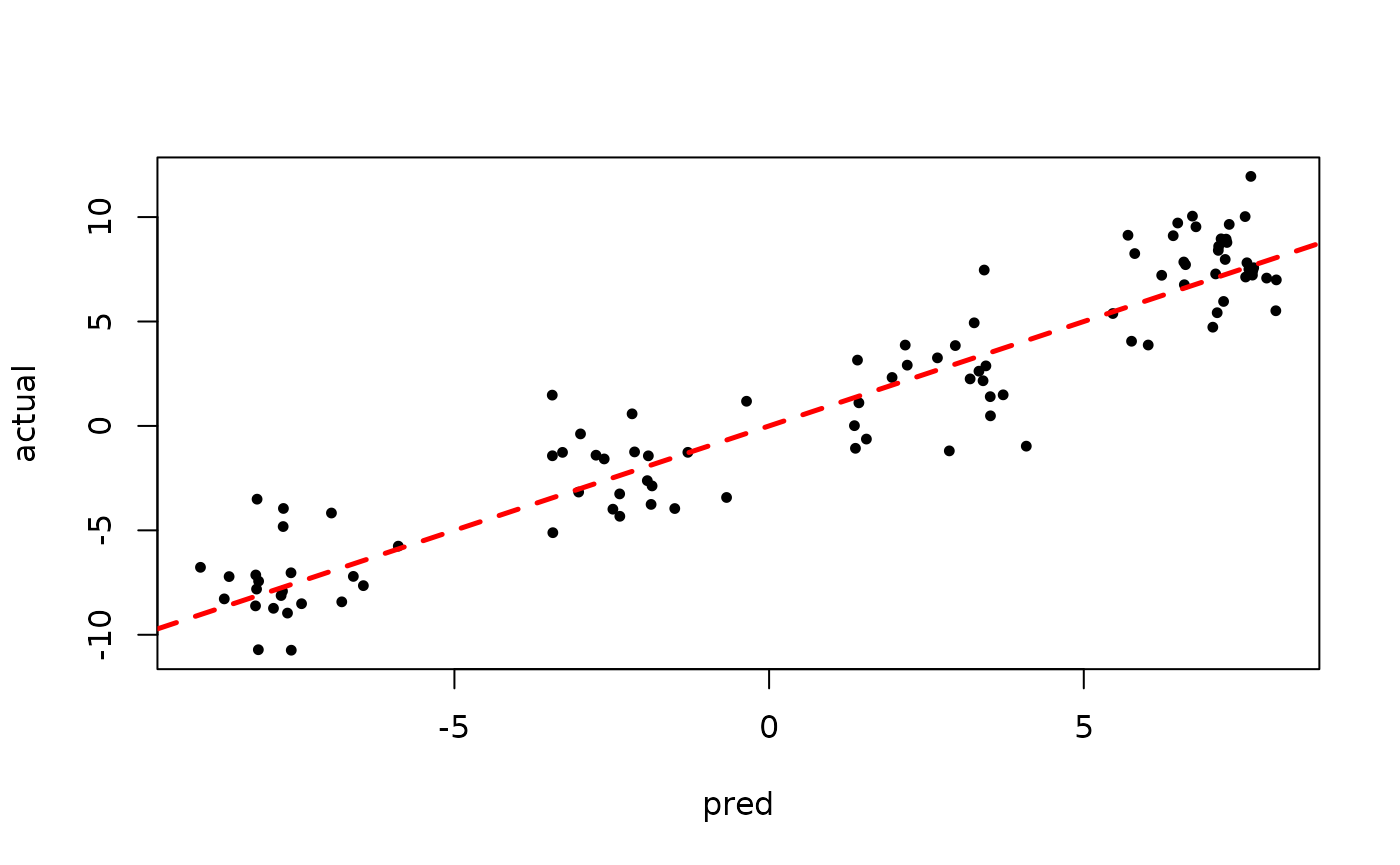

BART MCMC without Warmstart

Next, we sample from this ensemble model without any warm-start initialization.

num_gfr <- 0
num_burnin <- 100
num_mcmc <- 100
num_samples <- num_gfr + num_burnin + num_mcmc
bart_model_root <- stochtree::bart(
    X_train = X_train, y_train = y_train, X_test = X_test, 
    num_trees = 100, num_gfr = num_gfr, num_burnin = num_burnin, 
    num_mcmc = num_mcmc, sample_sigma = T, sample_tau = T
)

Inspect the MCMC samples

plot(bart_model_root$sigma2_samples, ylab="sigma^2")

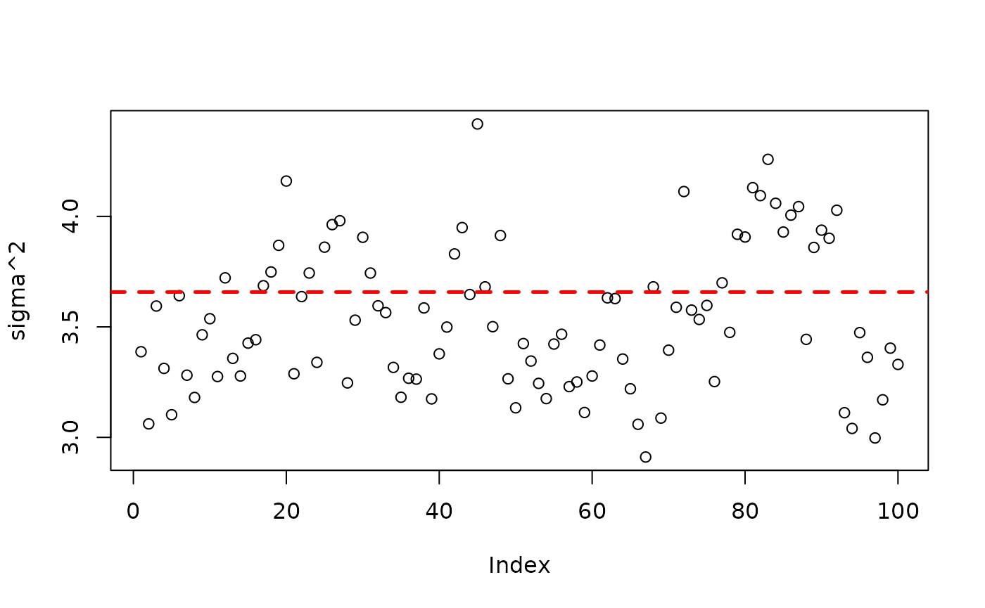
plot(rowMeans(bart_model_root$y_hat_test), y_test, 
     pch=16, cex=0.75, xlab = "pred", ylab = "actual")
abline(0,1,col="red",lty=2,lwd=2.5)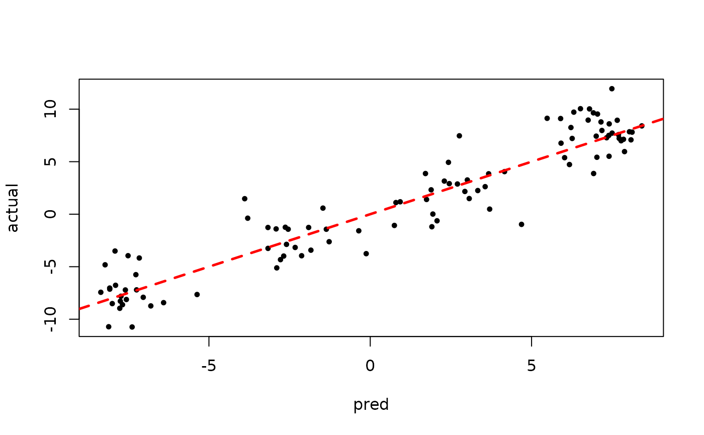

Demo 2: Partitioned Linear Model

Simulation

Here, we generate data from a simple partitioned linear model.

# Generate the data
n <- 500
p_x <- 10
p_w <- 1
snr <- 3
X <- matrix(runif(n*p_x), ncol = p_x)
W <- matrix(runif(n*p_w), ncol = p_w)
f_XW <- (
    ((0 <= X[,1]) & (0.25 > X[,1])) * (-7.5*W[,1]) + 
    ((0.25 <= X[,1]) & (0.5 > X[,1])) * (-2.5*W[,1]) + 
    ((0.5 <= X[,1]) & (0.75 > X[,1])) * (2.5*W[,1]) + 
    ((0.75 <= X[,1]) & (1 > X[,1])) * (7.5*W[,1])
)
noise_sd <- sd(f_XW) / snr
y <- f_XW + rnorm(n, 0, 1)*noise_sd

# Split data into test and train sets
test_set_pct <- 0.2
n_test <- round(test_set_pct*n)
n_train <- n - n_test
test_inds <- sort(sample(1:n, n_test, replace = FALSE))
train_inds <- (1:n)[!((1:n) %in% test_inds)]
X_test <- as.data.frame(X[test_inds,])
X_train <- as.data.frame(X[train_inds,])
W_test <- W[test_inds,]
W_train <- W[train_inds,]
y_test <- y[test_inds]
y_train <- y[train_inds]

Sampling and Analysis

Warmstart

We first sample from an ensemble model of $y \mid X$ using “warm-start” initialization samples (He and Hahn (2023)). This is the default in stochtree.

num_gfr <- 10
num_burnin <- 0
num_mcmc <- 100
num_samples <- num_gfr + num_burnin + num_mcmc
bart_model_warmstart <- stochtree::bart(
    X_train = X_train, W_train = W_train, y_train = y_train, 
    X_test = X_test, W_test = W_test, num_trees = 100, 
    num_gfr = num_gfr, num_burnin = num_burnin, 
    num_mcmc = num_mcmc, sample_sigma = T, sample_tau = T
)

Inspect the MCMC samples

plot(bart_model_warmstart$sigma2_samples, ylab="sigma^2")

plot(rowMeans(bart_model_warmstart$y_hat_test), y_test, 
     pch=16, cex=0.75, xlab = "pred", ylab = "actual")
abline(0,1,col="red",lty=2,lwd=2.5)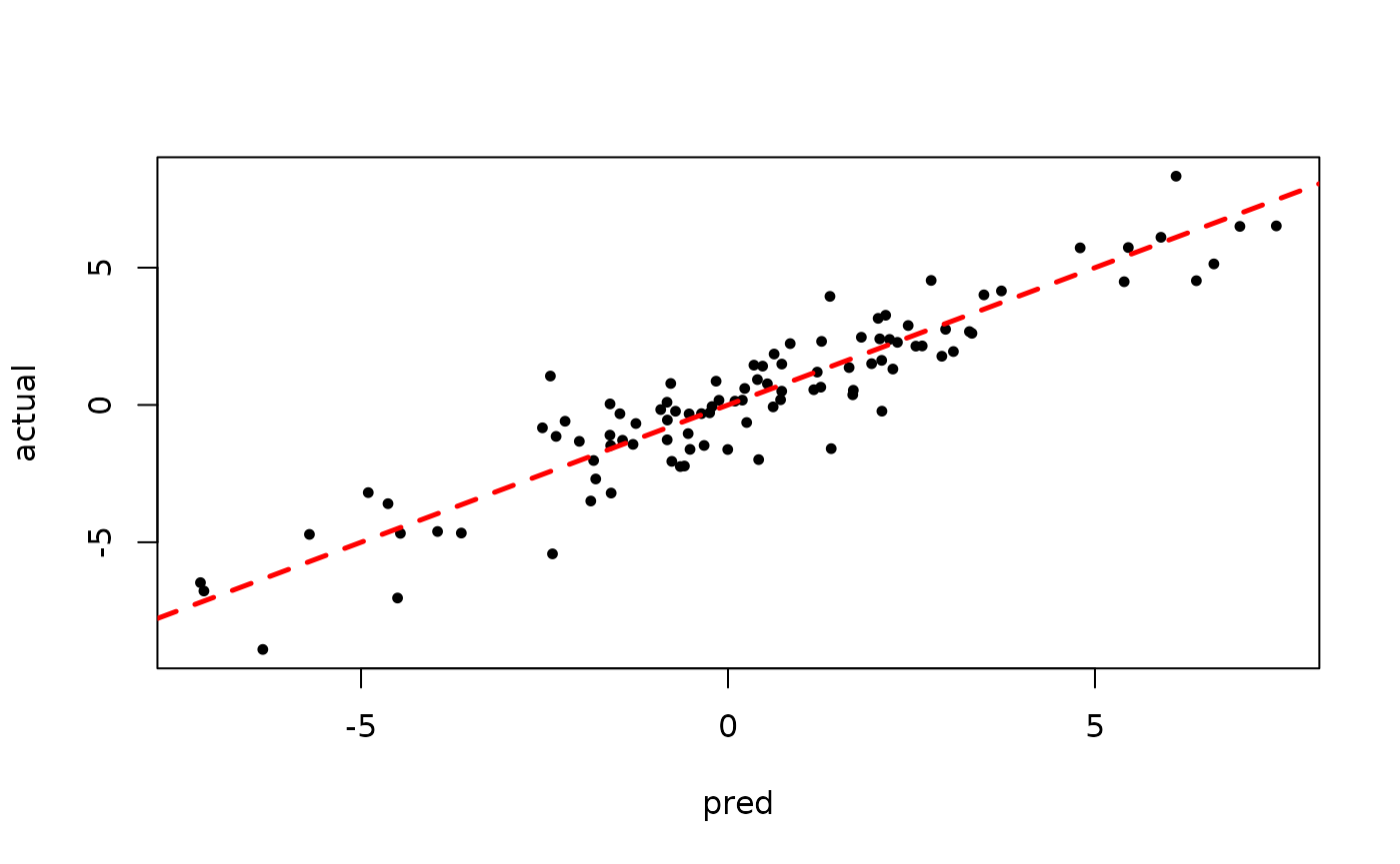

BART MCMC without Warmstart

Next, we sample from this ensemble model without any warm-start initialization.

num_gfr <- 0
num_burnin <- 100
num_mcmc <- 100
num_samples <- num_gfr + num_burnin + num_mcmc
bart_model_root <- stochtree::bart(
    X_train = X_train, W_train = W_train, y_train = y_train, 
    X_test = X_test, W_test = W_test, num_trees = 100, 
    num_gfr = num_gfr, num_burnin = num_burnin, 
    num_mcmc = num_mcmc, sample_sigma = T, sample_tau = T
)

Inspect the BART samples after burnin.

plot(bart_model_root$sigma2_samples, ylab="sigma^2")

plot(rowMeans(bart_model_root$y_hat_test), y_test, 
     pch=16, cex=0.75, xlab = "pred", ylab = "actual")
abline(0,1,col="red",lty=2,lwd=2.5)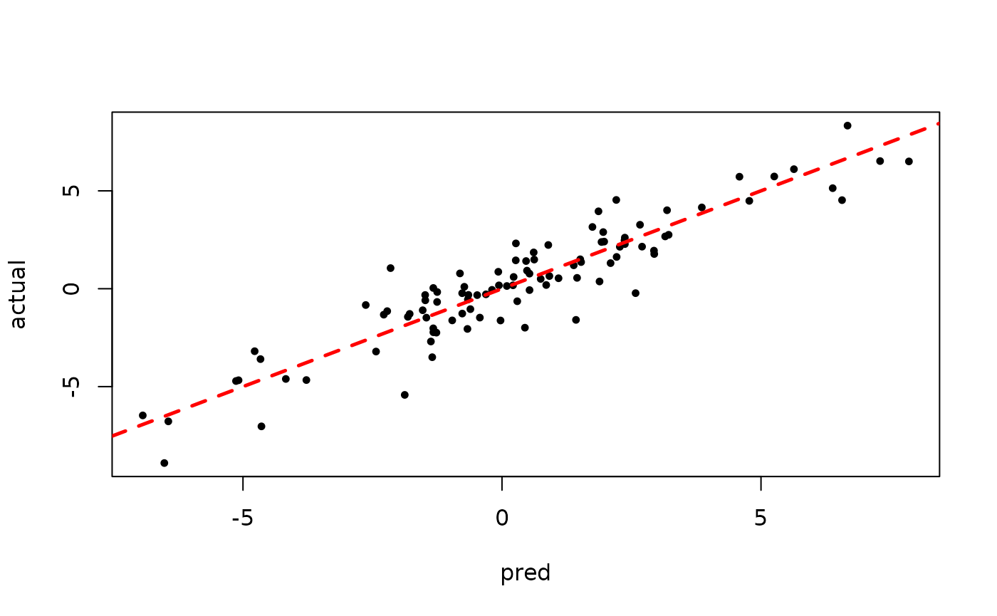

Demo 3: Partitioned Linear Model with Random Effects

Simulation

Here, we generate data from a simple partitioned linear model with an additive random effect structure.

# Generate the data
n <- 500
p_x <- 10
p_w <- 1
snr <- 3
X <- matrix(runif(n*p_x), ncol = p_x)
W <- matrix(runif(n*p_w), ncol = p_w)
group_ids <- rep(c(1,2), n %/% 2)
rfx_coefs <- matrix(c(-5, -3, 5, 3), nrow=2, byrow=TRUE)
rfx_basis <- cbind(1, runif(n, -1, 1))
f_XW <- (
    ((0 <= X[,1]) & (0.25 > X[,1])) * (-7.5*W[,1]) + 
    ((0.25 <= X[,1]) & (0.5 > X[,1])) * (-2.5*W[,1]) + 
    ((0.5 <= X[,1]) & (0.75 > X[,1])) * (2.5*W[,1]) + 
    ((0.75 <= X[,1]) & (1 > X[,1])) * (7.5*W[,1])
)
rfx_term <- rowSums(rfx_coefs[group_ids,] * rfx_basis)
noise_sd <- sd(f_XW) / snr
y <- f_XW + rfx_term + rnorm(n, 0, 1)*noise_sd

# Split data into test and train sets
test_set_pct <- 0.2
n_test <- round(test_set_pct*n)
n_train <- n - n_test
test_inds <- sort(sample(1:n, n_test, replace = FALSE))
train_inds <- (1:n)[!((1:n) %in% test_inds)]
X_test <- as.data.frame(X[test_inds,])
X_train <- as.data.frame(X[train_inds,])
W_test <- W[test_inds,]
W_train <- W[train_inds,]
y_test <- y[test_inds]
y_train <- y[train_inds]
group_ids_test <- group_ids[test_inds]
group_ids_train <- group_ids[train_inds]
rfx_basis_test <- rfx_basis[test_inds,]
rfx_basis_train <- rfx_basis[train_inds,]

Sampling and Analysis

Warmstart

We first sample from an ensemble model of $y \mid X$ using “warm-start” initialization samples (He and Hahn (2023)). This is the default in stochtree.

num_gfr <- 10
num_burnin <- 0
num_mcmc <- 100
num_samples <- num_gfr + num_burnin + num_mcmc
bart_model_warmstart <- stochtree::bart(
    X_train = X_train, W_train = W_train, y_train = y_train, 
    group_ids_train = group_ids_train, rfx_basis_train = rfx_basis_train, 
    X_test = X_test, W_test = W_test, group_ids_test = group_ids_test,
    rfx_basis_test = rfx_basis_test, num_trees = 100, num_gfr = num_gfr, 
    num_burnin = num_burnin, num_mcmc = num_mcmc, 
    sample_sigma = T, sample_tau = T
)

Inspect the MCMC samples

plot(bart_model_warmstart$sigma2_samples, ylab="sigma^2")
abline(h=noise_sd^2,col="red",lty=2,lwd=2.5)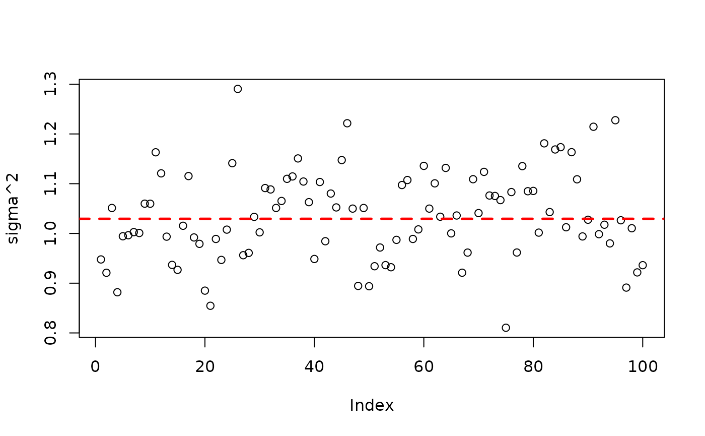

plot(rowMeans(bart_model_warmstart$y_hat_test), y_test, 
     pch=16, cex=0.75, xlab = "pred", ylab = "actual")
abline(0,1,col="red",lty=2,lwd=2.5)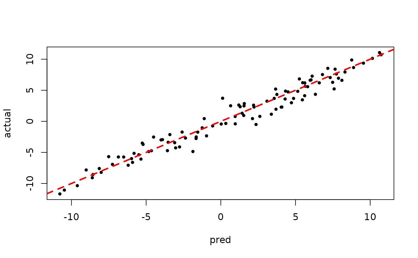

BART MCMC without Warmstart

Next, we sample from this ensemble model without any warm-start initialization.

num_gfr <- 0
num_burnin <- 100
num_mcmc <- 100
num_samples <- num_gfr + num_burnin + num_mcmc
bart_model_root <- stochtree::bart(
    X_train = X_train, W_train = W_train, y_train = y_train, 
    group_ids_train = group_ids_train, rfx_basis_train = rfx_basis_train, 
    X_test = X_test, W_test = W_test, group_ids_test = group_ids_test,
    rfx_basis_test = rfx_basis_test, num_trees = 100, num_gfr = num_gfr, 
    num_burnin = num_burnin, num_mcmc = num_mcmc, 
    sample_sigma = T, sample_tau = T
)

Inspect the MCMC samples

plot(bart_model_root$sigma2_samples, ylab="sigma^2")
abline(h=noise_sd^2,col="red",lty=2,lwd=2.5)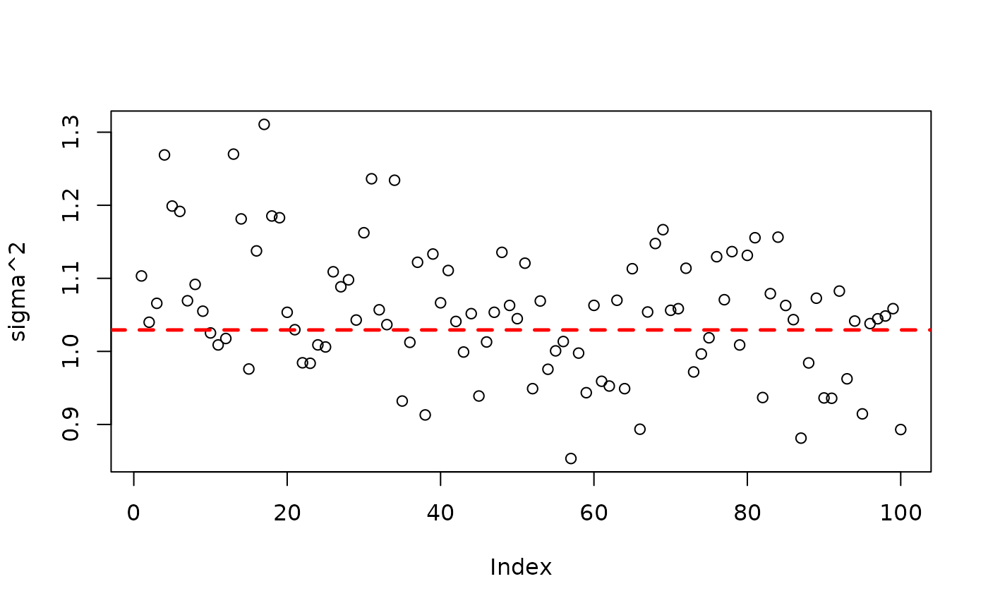

plot(rowMeans(bart_model_root$y_hat_test), y_test, 
     pch=16, cex=0.75, xlab = "pred", ylab = "actual")
abline(0,1,col="red",lty=2,lwd=2.5)

References

Chipman, Hugh A., Edward I. George, and Robert E. McCulloch. 2010. “BART: Bayesian additive regression trees.” The Annals of Applied Statistics 4 (1): 266–98. https://doi.org/10.1214/09-AOAS285.

He, Jingyu, and P Richard Hahn. 2023. “Stochastic Tree Ensembles for Regularized Nonlinear Regression.” Journal of the American Statistical Association 118 (541): 551–70.