Custom Sampling Routines in StochTree

Motivation

While the functions bart() and bcf() provide simple and performant interfaces for supervised learning / causal inference, stochtree also offers access to many of the “low-level” data structures that are typically implemented in C++. This low-level interface is not designed for performance or even simplicity — rather the intent is to provide a “prototype” interface to the C++ code that doesn’t require modifying any C++.

To illustrate when such a prototype interface might be useful, consider the classic BART algorithm:

   INPUT: $y$, $X$, $\tau$, $\nu$, $\lambda$, $\alpha$, $\beta$
   OUTPUT: $m$ samples of a decision forest with $k$ trees and global variance parameter $\sigma^2$
   Initialize $\sigma^2$ via a default or a data-dependent calibration exercise
   Initialize “forest 0” with $k$ trees with a single root node, referring to tree $j$’s prediction vector as $f_{0,j}$
   Compute residual as $r = y - \sum_{j=1}^k f_{0,j}$
   FOR $i$IN $\left\{1,\dots,m\right\}$:
      Initialize forest $i$ from forest $i-1$
      FOR $j$IN $\left\{1,\dots,k\right\}$:
         Add predictions for tree $j$ to residual: $r = r + f_{i,j}$
         Update tree $j$ via Metropolis-Hastings with $r$ and $X$ as data and tree priors depending on ($\tau$, $\sigma^2$, $\alpha$, $\beta$)
         Sample leaf node parameters for tree $j$ via Gibbs (leaf node prior is $N\left(0,\tau\right)$)
         Subtract (updated) predictions for tree $j$ from residual: $r = r - f_{i,j}$
      Sample $\sigma^2$ via Gibbs (prior is $IG(\nu/2,\nu\lambda/2)$)

While the algorithm itself is conceptually simple, much of the core computation is carried out in low-level languages such as C or C++ because of the tree data structure. As a result, any changes to this algorithm, such as supporting heteroskedasticity (Pratola et al. (2020)), categorical outcomes (Murray (2021)) or causal effect estimation (Hahn, Murray, and Carvalho (2020)) require modifying low-level code.

The prototype interface exposes the core components of the loop above at the R level, thus making it possible to interchange C++ computation for steps like “update tree $j$ via Metropolis-Hastings” with R computation for a custom variance model, other user-specified additive mean model components, and so on.

To begin, load the stochtree package

library(stochtree)

Demo 1: Supervised Learning

Simulation

Simulate a simple partitioned linear model

# Generate the data
n <- 500
p_X <- 10
p_W <- 1
X <- matrix(runif(n*p_X), ncol = p_X)
W <- matrix(runif(n*p_W), ncol = p_W)
f_XW <- (
    ((0 <= X[,1]) & (0.25 > X[,1])) * (-3*W[,1]) + 
    ((0.25 <= X[,1]) & (0.5 > X[,1])) * (-1*W[,1]) + 
    ((0.5 <= X[,1]) & (0.75 > X[,1])) * (1*W[,1]) + 
    ((0.75 <= X[,1]) & (1 > X[,1])) * (3*W[,1])
)
y <- f_XW + rnorm(n, 0, 1)

# Standardize outcome
y_bar <- mean(y)
y_std <- sd(y)
resid <- (y-y_bar)/y_std

Sampling

Set some parameters that inform the forest and variance parameter samplers

alpha <- 0.9
beta <- 1.25
min_samples_leaf <- 1
max_depth <- 10
num_trees <- 100
cutpoint_grid_size = 100
global_variance_init = 1.
tau_init = 0.5
leaf_prior_scale = matrix(c(tau_init), ncol = 1)
nu <- 4
lambda <- 0.5
a_leaf <- 2.
b_leaf <- 0.5
leaf_regression <- T
feature_types <- as.integer(rep(0, p_X)) # 0 = numeric
var_weights <- rep(1/p_X, p_X)

Initialize R-level access to the C++ classes needed to sample our model

# Data
if (leaf_regression) {
    forest_dataset <- createForestDataset(X, W)
    outcome_model_type <- 1
} else {
    forest_dataset <- createForestDataset(X)
    outcome_model_type <- 0
}
outcome <- createOutcome(resid)

# Random number generator (std::mt19937)
rng <- createRNG()

# Sampling data structures
forest_model <- createForestModel(forest_dataset, feature_types, 
                                  num_trees, n, alpha, beta, 
                                  min_samples_leaf, max_depth)

# "Active forest" (which gets updated by the sample) and 
# container of forest samples (which is written to when 
# a sample is not discarded due to burn-in / thinning)
if (leaf_regression) {
    forest_samples <- createForestContainer(num_trees, 1, F)
    active_forest <- createForest(num_trees, 1, F)
} else {
    forest_samples <- createForestContainer(num_trees, 1, T)
    active_forest <- createForest(num_trees, 1, T)
}

Prepare to run the sampler

num_warmstart <- 10
num_mcmc <- 100
num_samples <- num_warmstart + num_mcmc
global_var_samples <- c(global_variance_init, rep(0, num_samples))
leaf_scale_samples <- c(tau_init, rep(0, num_samples))

Run the grow-from-root sampler to “warm-start” BART

for (i in 1:num_warmstart) {
    # Sample forest
    forest_model$sample_one_iteration(
        forest_dataset, outcome, forest_samples, active_forest, rng, feature_types, 
        outcome_model_type, leaf_prior_scale, var_weights, 
        1, 1, global_var_samples[i], cutpoint_grid_size, keep_forest = T, gfr = T
    )
    
    # Sample global variance parameter
    global_var_samples[i+1] <- sample_sigma2_one_iteration(
        outcome, forest_dataset, rng, nu, lambda
    )
    
    # Sample leaf node variance parameter and update `leaf_prior_scale`
    leaf_scale_samples[i+1] <- sample_tau_one_iteration(
        active_forest, rng, a_leaf, b_leaf
    )
    leaf_prior_scale[1,1] <- leaf_scale_samples[i+1]
}

Pick up from the last GFR forest (and associated global variance / leaf scale parameters) with an MCMC sampler

for (i in (num_warmstart+1):num_samples) {
    # Sample forest
    forest_model$sample_one_iteration(
        forest_dataset, outcome, forest_samples, active_forest, rng, feature_types, 
        outcome_model_type, leaf_prior_scale, var_weights, 
        1, 1, global_var_samples[i], cutpoint_grid_size, keep_forest = T, gfr = F
    )
    
    # Sample global variance parameter
    global_var_samples[i+1] <- sample_sigma2_one_iteration(
        outcome, forest_dataset, rng, nu, lambda
    )
    
    # Sample leaf node variance parameter and update `leaf_prior_scale`
    leaf_scale_samples[i+1] <- sample_tau_one_iteration(
        active_forest, rng, a_leaf, b_leaf
    )
    leaf_prior_scale[1,1] <- leaf_scale_samples[i+1]
}

Predict and rescale samples

# Forest predictions
preds <- forest_samples$predict(forest_dataset)*y_std + y_bar

# Global error variance
sigma_samples <- sqrt(global_var_samples)*y_std

Results

Inspect the initial samples obtained via “grow-from-root” (He and Hahn (2023))

plot(sigma_samples[1:num_warmstart], ylab="sigma")

plot(rowMeans(preds[,1:num_warmstart]), y, pch=16, 
     cex=0.75, xlab = "pred", ylab = "actual")
abline(0,1,col="red",lty=2,lwd=2.5)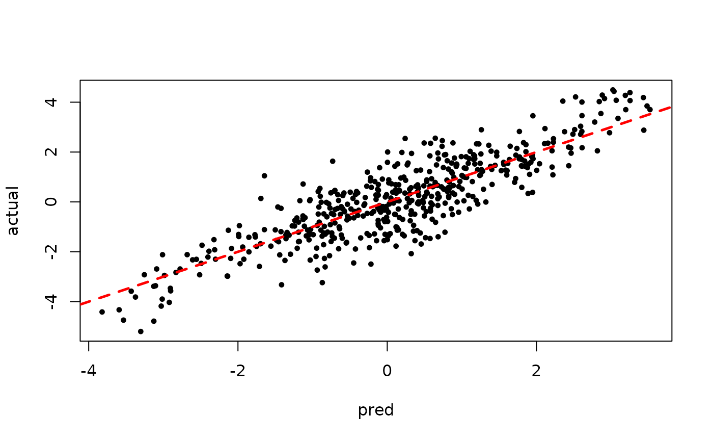

Inspect the BART samples obtained after “warm-starting”

plot(sigma_samples[(num_warmstart+1):num_samples], ylab="sigma")

plot(rowMeans(preds[,(num_warmstart+1):num_samples]), y, pch=16, 
     cex=0.75, xlab = "pred", ylab = "actual")
abline(0,1,col="red",lty=2,lwd=2.5)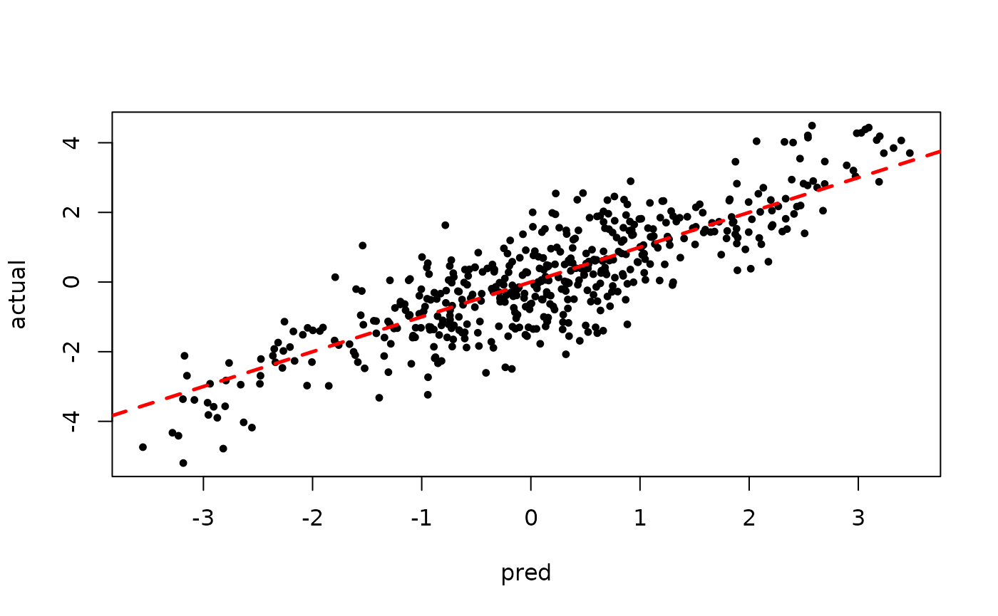

Demo 2: Supervised Learning with Additive Random Effects

We build on the above example and add a simple “random effects” structure: every observation is in either group 1 or group 2 and there is a random group intercept (simulated to be quite strong, underscoring the need for random effects modeling).

Simulation

Simulate a partitioned linear model with a simple additive group random effect structure

# Generate the data
n <- 500
p_X <- 10
p_W <- 1
X <- matrix(runif(n*p_X), ncol = p_X)
W <- matrix(runif(n*p_W), ncol = p_W)
group_ids <- rep(c(1,2), n %/% 2)
rfx_coefs <- c(-5, 5)
rfx_basis <- rep(1, n)
f_XW <- (
    ((0 <= X[,1]) & (0.25 > X[,1])) * (-3*W[,1]) + 
    ((0.25 <= X[,1]) & (0.5 > X[,1])) * (-1*W[,1]) + 
    ((0.5 <= X[,1]) & (0.75 > X[,1])) * (1*W[,1]) + 
    ((0.75 <= X[,1]) & (1 > X[,1])) * (3*W[,1])
)
rfx_term <- rfx_coefs[group_ids] * rfx_basis
y <- f_XW + rfx_term + rnorm(n, 0, 1)

# Standardize outcome
y_bar <- mean(y)
y_std <- sd(y)
resid <- (y-y_bar)/y_std

Sampling

Set some parameters that inform the forest and variance parameter samplers

alpha <- 0.9
beta <- 1.25
min_samples_leaf <- 1
max_depth <- 10
num_trees <- 100
cutpoint_grid_size = 100
global_variance_init = 1.
tau_init = 0.5
leaf_prior_scale = matrix(c(tau_init), ncol = 1)
nu <- 4
lambda <- 0.5
a_leaf <- 2.
b_leaf <- 0.5
leaf_regression <- T
feature_types <- as.integer(rep(0, p_X)) # 0 = numeric
var_weights <- rep(1/p_X, p_X)

Set some parameters that inform the random effects samplers

alpha_init <- c(1)
xi_init <- matrix(c(1,1),1,2)
sigma_alpha_init <- matrix(c(1),1,1)
sigma_xi_init <- matrix(c(1),1,1)
sigma_xi_shape <- 1
sigma_xi_scale <- 1

Initialize R-level access to the C++ classes needed to sample our model

# Data
if (leaf_regression) {
    forest_dataset <- createForestDataset(X, W)
    outcome_model_type <- 1
} else {
    forest_dataset <- createForestDataset(X)
    outcome_model_type <- 0
}
outcome <- createOutcome(resid)

# Random number generator (std::mt19937)
rng <- createRNG()

# Sampling data structures
forest_model <- createForestModel(forest_dataset, feature_types, 
                                  num_trees, n, alpha, beta, 
                                  min_samples_leaf, max_depth)

# "Active forest" (which gets updated by the sample) and 
# container of forest samples (which is written to when 
# a sample is not discarded due to burn-in / thinning)
if (leaf_regression) {
    forest_samples <- createForestContainer(num_trees, 1, F)
    active_forest <- createForest(num_trees, 1, F)
} else {
    forest_samples <- createForestContainer(num_trees, 1, T)
    active_forest <- createForest(num_trees, 1, T)
}

# Random effects dataset
rfx_basis <- as.matrix(rfx_basis)
group_ids <- as.integer(group_ids)
rfx_dataset <- createRandomEffectsDataset(group_ids, rfx_basis)

# Random effects details
num_groups <- length(unique(group_ids))
num_components <- ncol(rfx_basis)

# Random effects tracker
rfx_tracker <- createRandomEffectsTracker(group_ids)

# Random effects model
rfx_model <- createRandomEffectsModel(num_components, num_groups)
rfx_model$set_working_parameter(alpha_init)
rfx_model$set_group_parameters(xi_init)
rfx_model$set_working_parameter_cov(sigma_alpha_init)
rfx_model$set_group_parameter_cov(sigma_xi_init)
rfx_model$set_variance_prior_shape(sigma_xi_shape)
rfx_model$set_variance_prior_scale(sigma_xi_scale)

# Random effect samples
rfx_samples <- createRandomEffectSamples(num_components, num_groups, rfx_tracker)

Prepare to run the sampler

num_warmstart <- 10
num_mcmc <- 100
num_samples <- num_warmstart + num_mcmc
global_var_samples <- c(global_variance_init, rep(0, num_samples))
leaf_scale_samples <- c(tau_init, rep(0, num_samples))

Run the grow-from-root sampler to “warm-start” BART

for (i in 1:num_warmstart) {
    # Sample forest
    forest_model$sample_one_iteration(
        forest_dataset, outcome, forest_samples, active_forest, rng, feature_types, 
        outcome_model_type, leaf_prior_scale, var_weights, 
        1, 1, global_var_samples[i], cutpoint_grid_size, keep_forest = T, gfr = T
    )
    
    # Sample global variance parameter
    global_var_samples[i+1] <- sample_sigma2_one_iteration(
        outcome, forest_dataset, rng, nu, lambda
    )
    
    # Sample leaf node variance parameter and update `leaf_prior_scale`
    leaf_scale_samples[i+1] <- sample_tau_one_iteration(
        active_forest, rng, a_leaf, b_leaf
    )
    leaf_prior_scale[1,1] <- leaf_scale_samples[i+1]
    
    # Sample random effects model
    rfx_model$sample_random_effect(rfx_dataset, outcome, rfx_tracker, rfx_samples, 
                                   TRUE, global_var_samples[i+1], rng)
}

Pick up from the last GFR forest (and associated global variance / leaf scale parameters) with an MCMC sampler

for (i in (num_warmstart+1):num_samples) {
    # Sample forest
    forest_model$sample_one_iteration(
        forest_dataset, outcome, forest_samples, active_forest, rng, feature_types, 
        outcome_model_type, leaf_prior_scale, var_weights, 
        1, 1, global_var_samples[i], cutpoint_grid_size, keep_forest = T, gfr = F
    )
    
    # Sample global variance parameter
    global_var_samples[i+1] <- sample_sigma2_one_iteration(
        outcome, forest_dataset, rng, nu, lambda
    )
    
    # Sample leaf node variance parameter and update `leaf_prior_scale`
    leaf_scale_samples[i+1] <- sample_tau_one_iteration(
        active_forest, rng, a_leaf, b_leaf
    )
    leaf_prior_scale[1,1] <- leaf_scale_samples[i+1]
    
    # Sample random effects model
    rfx_model$sample_random_effect(rfx_dataset, outcome, rfx_tracker, rfx_samples, 
                                   TRUE, global_var_samples[i+1], rng)
}

Predict and rescale samples

# Forest predictions
forest_preds <- forest_samples$predict(forest_dataset)*y_std + y_bar

# Random effects predictions
rfx_preds <- rfx_samples$predict(group_ids, rfx_basis)*y_std

# Overall predictions
preds <- forest_preds + rfx_preds

# Global error variance
sigma_samples <- sqrt(global_var_samples)*y_std

Results

Inspect the initial samples obtained via grow-from-root and an additive random effects model

plot(sigma_samples[1:num_warmstart], ylab="sigma")

plot(rowMeans(preds[,1:num_warmstart]), y, pch=16, 
     cex=0.75, xlab = "pred", ylab = "actual")
abline(0,1,col="red",lty=2,lwd=2.5)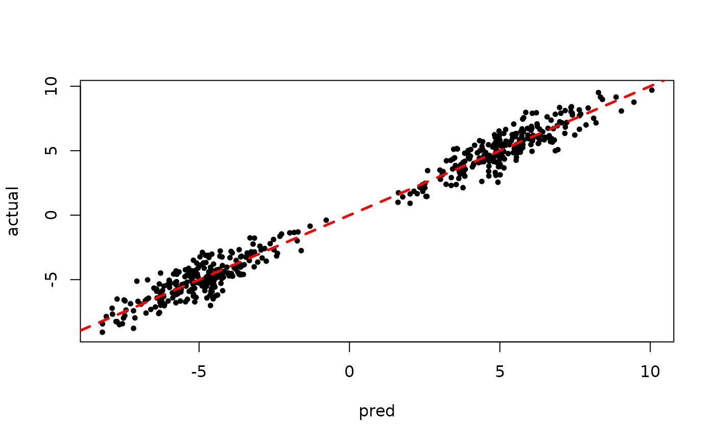

Inspect the BART samples obtained after “warm-starting” plus an additive random effects model

plot(sigma_samples[(num_warmstart+1):num_samples], ylab="sigma")

plot(rowMeans(preds[,(num_warmstart+1):num_samples]), y, pch=16, 
     cex=0.75, xlab = "pred", ylab = "actual")
abline(0,1,col="red",lty=2,lwd=2.5)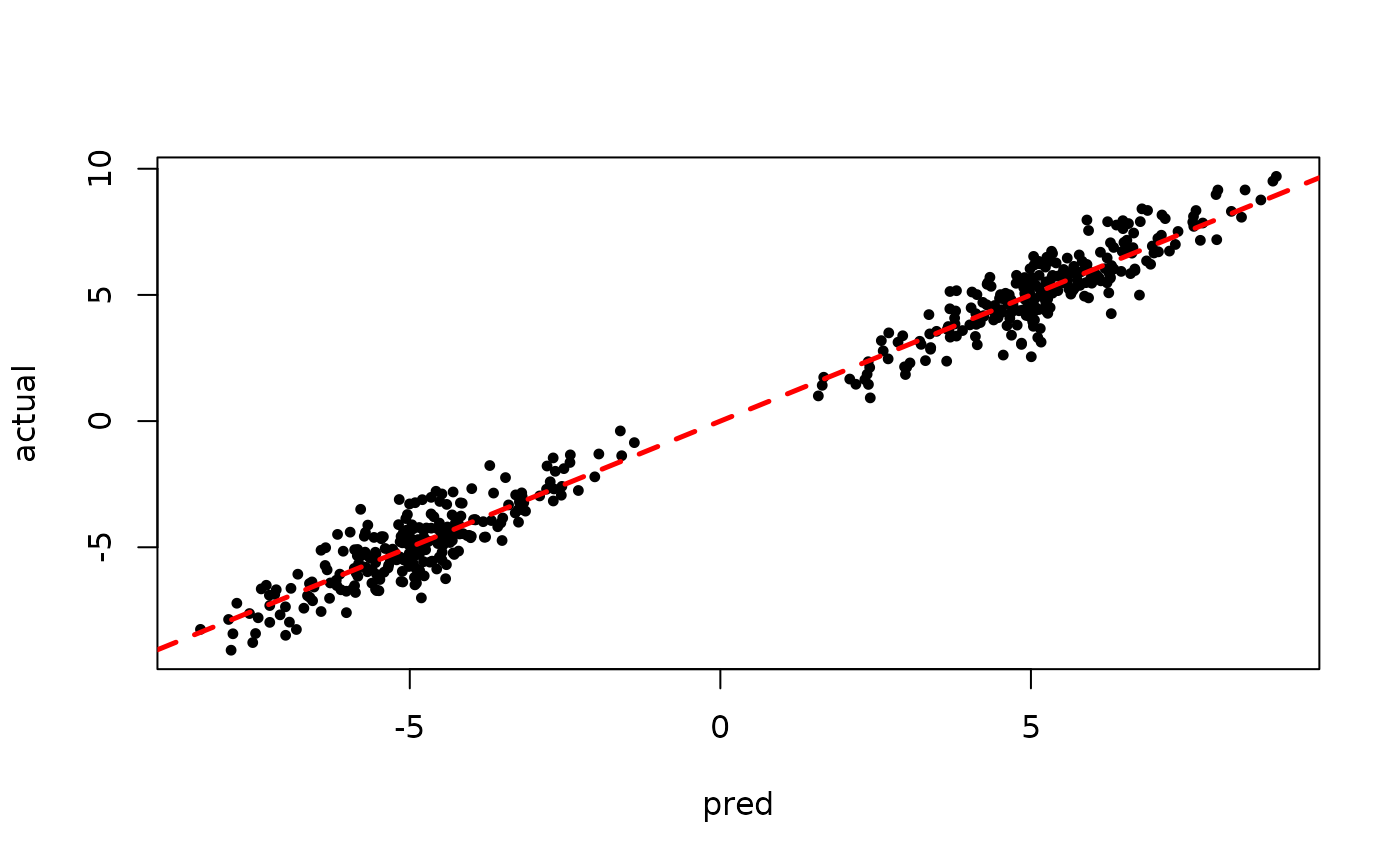

Now inspect the samples from the BART forest alone (without considering the random effect predictions)

plot(rowMeans(forest_preds[,(num_warmstart+1):num_samples]), y, pch=16, 
     cex=0.75, xlab = "pred", ylab = "actual")
abline(0,1,col="red",lty=2,lwd=2.5)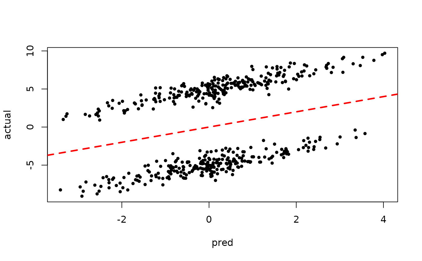

Demo 3: Supervised Learning with Additive Multi-Component Random Effects

We build once again on the above example, in this case allowing for a random intercept and regression coefficient (on a pre-specified basis) for each group (1 and 2).

Simulation

Simulate a partitioned linear model with a simple additive group random effect structure

# Generate the data
n <- 500
p_X <- 10
p_W <- 1
X <- matrix(runif(n*p_X), ncol = p_X)
W <- matrix(runif(n*p_W), ncol = p_W)
group_ids <- rep(c(1,2), n %/% 2)
rfx_coefs <- matrix(c(-5, -3, 5, 3), nrow=2, byrow=TRUE)
rfx_basis <- cbind(1, runif(n, -1, 1))
f_XW <- (
    ((0 <= X[,1]) & (0.25 > X[,1])) * (-3*W[,1]) + 
    ((0.25 <= X[,1]) & (0.5 > X[,1])) * (-1*W[,1]) + 
    ((0.5 <= X[,1]) & (0.75 > X[,1])) * (1*W[,1]) + 
    ((0.75 <= X[,1]) & (1 > X[,1])) * (3*W[,1])
)
rfx_term <- rowSums(rfx_coefs[group_ids,] * rfx_basis)
y <- f_XW + rfx_term + rnorm(n, 0, 1)

# Standardize outcome
y_bar <- mean(y)
y_std <- sd(y)
resid <- (y-y_bar)/y_std

Sampling

Set some parameters that inform the forest and variance parameter samplers

alpha <- 0.9
beta <- 1.25
min_samples_leaf <- 1
max_depth <- 10
num_trees <- 100
cutpoint_grid_size = 100
global_variance_init = 1.
tau_init = 0.5
leaf_prior_scale = matrix(c(tau_init), ncol = 1)
nu <- 4
lambda <- 0.5
a_leaf <- 2.
b_leaf <- 0.5
leaf_regression <- T
feature_types <- as.integer(rep(0, p_X)) # 0 = numeric
var_weights <- rep(1/p_X, p_X)

Set some parameters that inform the random effects samplers

alpha_init <- c(1,0)
xi_init <- matrix(c(1,0,1,0),2,2)
sigma_alpha_init <- diag(1,2,2)
sigma_xi_init <- diag(1,2,2)
sigma_xi_shape <- 1
sigma_xi_scale <- 1

Initialize R-level access to the C++ classes needed to sample our model

# Data
if (leaf_regression) {
    forest_dataset <- createForestDataset(X, W)
    outcome_model_type <- 1
} else {
    forest_dataset <- createForestDataset(X)
    outcome_model_type <- 0
}
outcome <- createOutcome(resid)

# Random number generator (std::mt19937)
rng <- createRNG()

# Sampling data structures
forest_model <- createForestModel(forest_dataset, feature_types, 
                                  num_trees, n, alpha, beta, 
                                  min_samples_leaf, max_depth)

# "Active forest" (which gets updated by the sample) and 
# container of forest samples (which is written to when 
# a sample is not discarded due to burn-in / thinning)
if (leaf_regression) {
    forest_samples <- createForestContainer(num_trees, 1, F)
    active_forest <- createForest(num_trees, 1, F)
} else {
    forest_samples <- createForestContainer(num_trees, 1, T)
    active_forest <- createForest(num_trees, 1, T)
}

# Random effects dataset
rfx_basis <- as.matrix(rfx_basis)
group_ids <- as.integer(group_ids)
rfx_dataset <- createRandomEffectsDataset(group_ids, rfx_basis)

# Random effects details
num_groups <- length(unique(group_ids))
num_components <- ncol(rfx_basis)

# Random effects tracker
rfx_tracker <- createRandomEffectsTracker(group_ids)

# Random effects model
rfx_model <- createRandomEffectsModel(num_components, num_groups)
rfx_model$set_working_parameter(alpha_init)
rfx_model$set_group_parameters(xi_init)
rfx_model$set_working_parameter_cov(sigma_alpha_init)
rfx_model$set_group_parameter_cov(sigma_xi_init)
rfx_model$set_variance_prior_shape(sigma_xi_shape)
rfx_model$set_variance_prior_scale(sigma_xi_scale)

# Random effect samples
rfx_samples <- createRandomEffectSamples(num_components, num_groups, rfx_tracker)

Prepare to run the sampler

num_warmstart <- 10
num_mcmc <- 100
num_samples <- num_warmstart + num_mcmc
global_var_samples <- c(global_variance_init, rep(0, num_samples))
leaf_scale_samples <- c(tau_init, rep(0, num_samples))

Run the grow-from-root sampler to “warm-start” BART

for (i in 1:num_warmstart) {
    # Sample forest
    forest_model$sample_one_iteration(
        forest_dataset, outcome, forest_samples, active_forest, rng, feature_types, 
        outcome_model_type, leaf_prior_scale, var_weights, 
        1, 1, global_var_samples[i], cutpoint_grid_size, keep_forest = T, gfr = T
    )
    
    # Sample global variance parameter
    global_var_samples[i+1] <- sample_sigma2_one_iteration(
        outcome, forest_dataset, rng, nu, lambda
    )
    
    # Sample leaf node variance parameter and update `leaf_prior_scale`
    leaf_scale_samples[i+1] <- sample_tau_one_iteration(
        active_forest, rng, a_leaf, b_leaf
    )
    leaf_prior_scale[1,1] <- leaf_scale_samples[i+1]
    
    # Sample random effects model
    rfx_model$sample_random_effect(rfx_dataset, outcome, rfx_tracker, rfx_samples, 
                                   TRUE, global_var_samples[i+1], rng)
}

Pick up from the last GFR forest (and associated global variance / leaf scale parameters) with an MCMC sampler

for (i in (num_warmstart+1):num_samples) {
    # Sample forest
    forest_model$sample_one_iteration(
        forest_dataset, outcome, forest_samples, active_forest, rng, feature_types, 
        outcome_model_type, leaf_prior_scale, var_weights, 
        1, 1, global_var_samples[i], cutpoint_grid_size, keep_forest = T, gfr = F
    )
    
    # Sample global variance parameter
    global_var_samples[i+1] <- sample_sigma2_one_iteration(
        outcome, forest_dataset, rng, nu, lambda
    )
    
    # Sample leaf node variance parameter and update `leaf_prior_scale`
    leaf_scale_samples[i+1] <- sample_tau_one_iteration(
        active_forest, rng, a_leaf, b_leaf
    )
    leaf_prior_scale[1,1] <- leaf_scale_samples[i+1]
    
    # Sample random effects model
    rfx_model$sample_random_effect(rfx_dataset, outcome, rfx_tracker, rfx_samples, 
                                   TRUE, global_var_samples[i+1], rng)
}

Predict and rescale samples

# Forest predictions
forest_preds <- forest_samples$predict(forest_dataset)*y_std + y_bar

# Random effects predictions
rfx_preds <- rfx_samples$predict(group_ids, rfx_basis)*y_std

# Overall predictions
preds <- forest_preds + rfx_preds

# Global error variance
sigma_samples <- sqrt(global_var_samples)*y_std

Results

Inspect the initial samples obtained via grow-from-root and an additive random effects model

plot(sigma_samples[1:num_warmstart], ylab="sigma")

plot(rowMeans(preds[,1:num_warmstart]), y, pch=16, 
     cex=0.75, xlab = "pred", ylab = "actual")
abline(0,1,col="red",lty=2,lwd=2.5)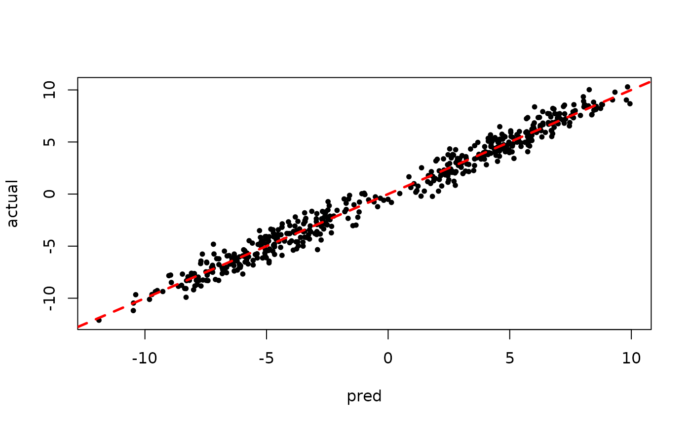

Inspect the BART samples obtained after “warm-starting” plus an additive random effects model

plot(sigma_samples[(num_warmstart+1):num_samples], ylab="sigma")

plot(rowMeans(preds[,(num_warmstart+1):num_samples]), y, pch=16, 
     cex=0.75, xlab = "pred", ylab = "actual")
abline(0,1,col="red",lty=2,lwd=2.5)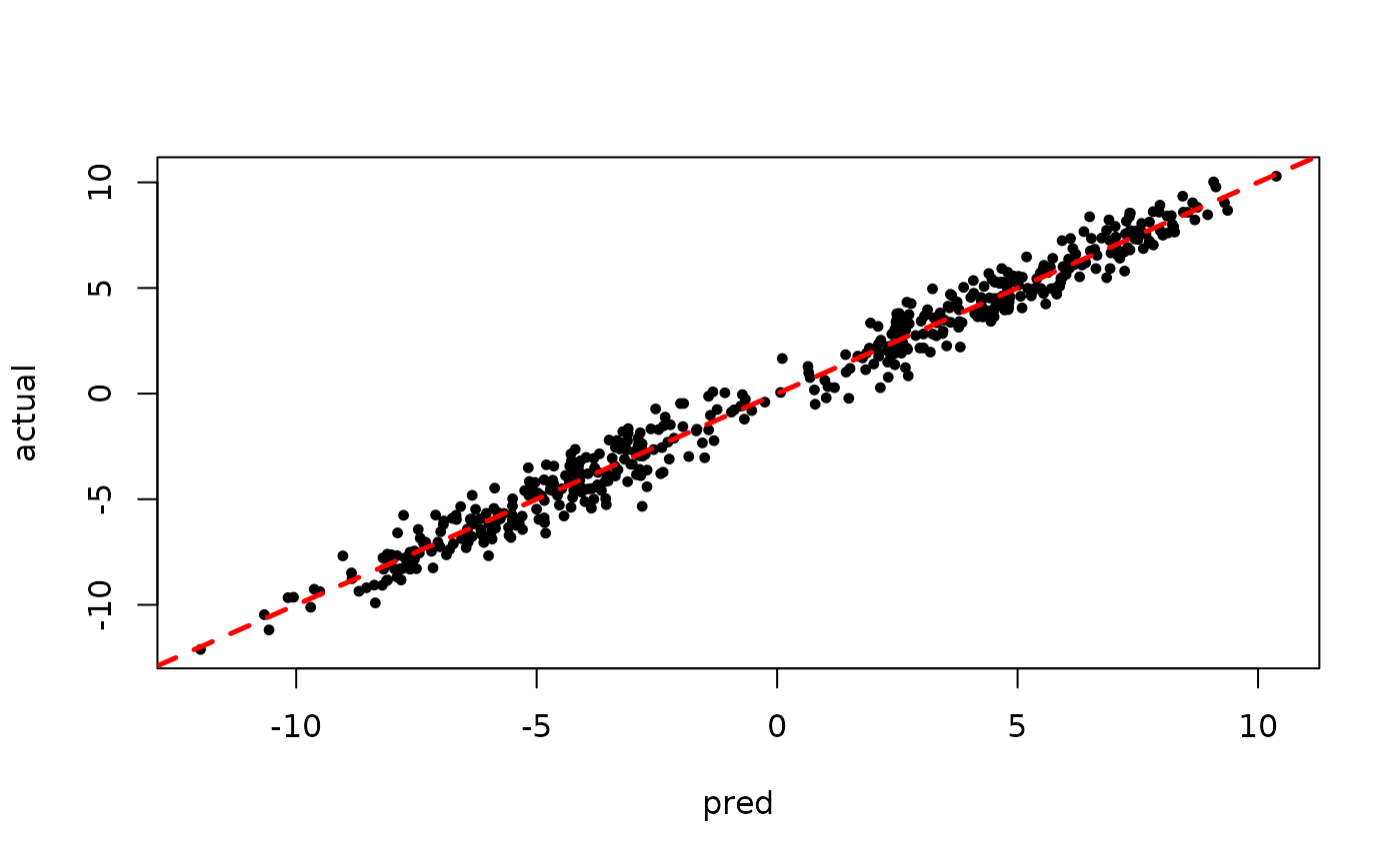

Now inspect the samples from the BART forest alone (without considering the random effect predictions)

plot(rowMeans(forest_preds[,(num_warmstart+1):num_samples]), y, pch=16, 
     cex=0.75, xlab = "pred", ylab = "actual")
abline(0,1,col="red",lty=2,lwd=2.5)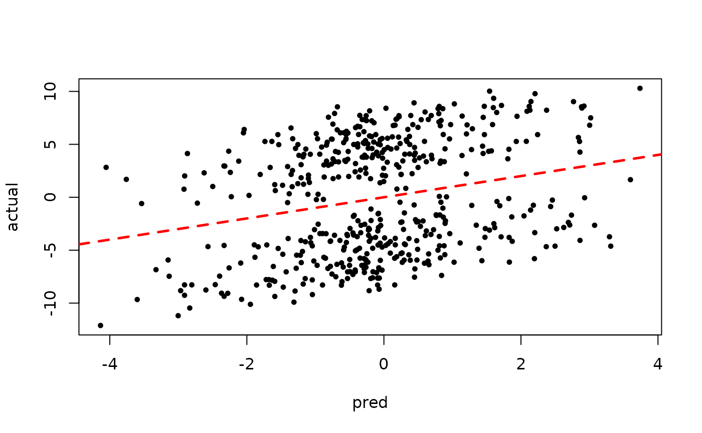

Demo 4: Supervised Learning with Additive Linear Model

Instead of group random effects, here we show how to combine a stochastic forest with an additive linear regression term. The model corresponds broadly to

$$\begin{equation*} \begin{aligned} y &= W\beta + f(X) + \epsilon\\ f(X) &\sim \text{BART}(c,d)\\ \beta &\sim \mathcal{N}(0, \tau)\\ \epsilon &\sim \mathcal{N}\left(0,\sigma^2\right)\\ \sigma^2 &\sim \text{IG}(a,b) \end{aligned} \end{equation*}$$

Simulation

Simulate a partitioned linear model with a simple additive group random effect structure

# Generate the data
n <- 500
p_X <- 10
p_W <- 1
X <- matrix(runif(n*p_X), ncol = p_X)
W <- matrix(runif(n*p_W), ncol = p_W)
beta_W <- c(5)
f_XW <- (
    ((0 <= X[,1]) & (0.25 > X[,1])) * (-3) + 
    ((0.25 <= X[,1]) & (0.5 > X[,1])) * (-1) + 
    ((0.5 <= X[,1]) & (0.75 > X[,1])) * (1) + 
    ((0.75 <= X[,1]) & (1 > X[,1])) * (3)
)
lm_term <- W %*% beta_W
y <- lm_term + f_XW + rnorm(n, 0, 1)

# Standardize outcome
y_bar <- mean(y)
y_std <- sd(y)
resid <- (y-y_bar)/y_std

Sampling

Set some parameters that inform the forest and variance parameter samplers

alpha_bart <- 0.9
beta_bart <- 1.25
min_samples_leaf <- 1
max_depth <- 10
num_trees <- 100
cutpoint_grid_size = 100
global_variance_init = 1.
tau_init = 0.5
leaf_prior_scale = matrix(c(tau_init), ncol = 1)
nu <- 4
lambda <- 0.5
a_leaf <- 2.
b_leaf <- 0.5
leaf_regression <- F
feature_types <- as.integer(rep(0, p_X)) # 0 = numeric
var_weights <- rep(1/p_X, p_X)
beta_tau <- 20

Initialize R-level access to the C++ classes needed to sample our model

# Data
if (leaf_regression) {
    forest_dataset <- createForestDataset(X, W)
    outcome_model_type <- 1
} else {
    forest_dataset <- createForestDataset(X)
    outcome_model_type <- 0
}
outcome <- createOutcome(resid)

# Random number generator (std::mt19937)
rng <- createRNG()

# Sampling data structures
forest_model <- createForestModel(forest_dataset, feature_types, 
                                  num_trees, n, alpha_bart, beta_bart, 
                                  min_samples_leaf, max_depth)

# "Active forest" (which gets updated by the sample) and 
# container of forest samples (which is written to when 
# a sample is not discarded due to burn-in / thinning)
if (leaf_regression) {
    forest_samples <- createForestContainer(num_trees, 1, F)
    active_forest <- createForest(num_trees, 1, F)
} else {
    forest_samples <- createForestContainer(num_trees, 1, T)
    active_forest <- createForest(num_trees, 1, T)
}

Prepare to run the sampler

num_warmstart <- 20
num_mcmc <- 100
num_samples <- num_warmstart + num_mcmc
beta_init <- 0
global_var_samples <- c(global_variance_init, rep(0, num_samples))
leaf_scale_samples <- c(tau_init, rep(0, num_samples))
beta_samples <- c(beta_init, rep(0, num_samples))

Run the grow-from-root sampler to “warm-start” BART

for (i in 1:num_warmstart) {
    # Initialize vectors needed for posterior sampling
    if (i == 1) {
        beta_hat <- beta_init
        yhat_forest <- rep(0, n)
        partial_res <- resid - yhat_forest
    } else {
        yhat_forest <- forest_samples$predict_raw_single_forest(forest_dataset, (i-1)-1)
        partial_res <- resid - yhat_forest
        outcome$add_vector(W %*% beta_hat)
    }
    # Sample beta from bayesian linear model with gaussian prior
    sigma2 <- global_var_samples[i]
    beta_posterior_mean <- sum(partial_res*W[,1])/(sigma2 + sum(W[,1]*W[,1]))
    beta_posterior_var <- (sigma2*beta_tau)/(sigma2 + sum(W[,1]*W[,1]))
    beta_hat <- rnorm(1, beta_posterior_mean, sqrt(beta_posterior_var))
    beta_samples[i+1] <- beta_hat
    # Update partial residual before sampling forest
    outcome$subtract_vector(W %*% beta_hat)
    
    # Sample forest
    forest_model$sample_one_iteration(
        forest_dataset, outcome, forest_samples, active_forest, rng, feature_types, 
        outcome_model_type, leaf_prior_scale, var_weights, 
        1, 1, sigma2, cutpoint_grid_size, keep_forest = T, gfr = T
    )
    
    # Sample global variance parameter
    global_var_samples[i+1] <- sample_sigma2_one_iteration(
        outcome, forest_dataset, rng, nu, lambda
    )
}

Pick up from the last GFR forest (and associated global variance / leaf scale parameters) with an MCMC sampler

for (i in (num_warmstart+1):num_samples) {
    # Initialize vectors needed for posterior sampling
    if (i == 1) {
        beta_hat <- beta_init
        yhat_forest <- rep(0, n)
        partial_res <- resid - yhat_forest
    } else {
        yhat_forest <- forest_samples$predict_raw_single_forest(forest_dataset, (i-1)-1)
        partial_res <- resid - yhat_forest
        outcome$add_vector(W %*% beta_hat)
    }
    # Sample beta from bayesian linear model with gaussian prior
    sigma2 <- global_var_samples[i]
    beta_posterior_mean <- sum(partial_res*W[,1])/(sigma2 + sum(W[,1]*W[,1]))
    beta_posterior_var <- (sigma2*beta_tau)/(sigma2 + sum(W[,1]*W[,1]))
    beta_hat <- rnorm(1, beta_posterior_mean, sqrt(beta_posterior_var))
    beta_samples[i+1] <- beta_hat
    # Update partial residual before sampling forest
    outcome$subtract_vector(W %*% beta_hat)
    
    # Sample forest
    forest_model$sample_one_iteration(
        forest_dataset, outcome, forest_samples, active_forest, rng, feature_types, 
        outcome_model_type, leaf_prior_scale, var_weights, 
        1, 1, global_var_samples[i], cutpoint_grid_size, keep_forest = T, gfr = F
    )
    
    # Sample global variance parameter
    global_var_samples[i+1] <- sample_sigma2_one_iteration(
        outcome, forest_dataset, rng, nu, lambda
    )
}

Predict and rescale samples

# Linear model predictions
lm_preds <- (sapply(1:num_samples, function(x) W[,1]*beta_samples[x+1]))*y_std

# Forest predictions
forest_preds <- forest_samples$predict(forest_dataset)*y_std + y_bar

# Overall predictions
preds <- forest_preds + lm_preds

# Global error variance
sigma_samples <- sqrt(global_var_samples)*y_std

# Regression parameter
beta_samples <- beta_samples*y_std

Results

Inspect the initial samples obtained via grow-from-root and an additive random effects model

plot(sigma_samples[1:num_warmstart], ylab="sigma")

plot(beta_samples[1:num_warmstart], ylab="beta")

plot(rowMeans(preds[,1:num_warmstart]), y, pch=16, 
     cex=0.75, xlab = "pred", ylab = "actual")
abline(0,1,col="red",lty=2,lwd=2.5)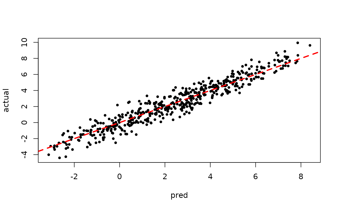

Inspect the BART samples obtained after “warm-starting” plus an additive random effects model

plot(sigma_samples[(num_warmstart+1):num_samples], ylab="sigma")

plot(beta_samples[(num_warmstart+1):num_samples], ylab="beta")

plot(rowMeans(preds[,(num_warmstart+1):num_samples]), y, pch=16, 
     cex=0.75, xlab = "pred", ylab = "actual")
abline(0,1,col="red",lty=2,lwd=2.5)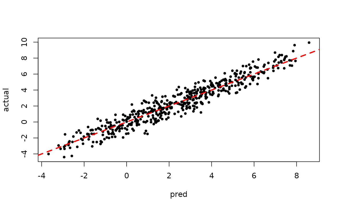

Now inspect the samples from the BART forest alone (without considering the additive linear model predictions)

plot(rowMeans(forest_preds[,(num_warmstart+1):num_samples]), y, pch=16, 
     cex=0.75, xlab = "pred", ylab = "actual")
abline(0,1,col="red",lty=2,lwd=2.5)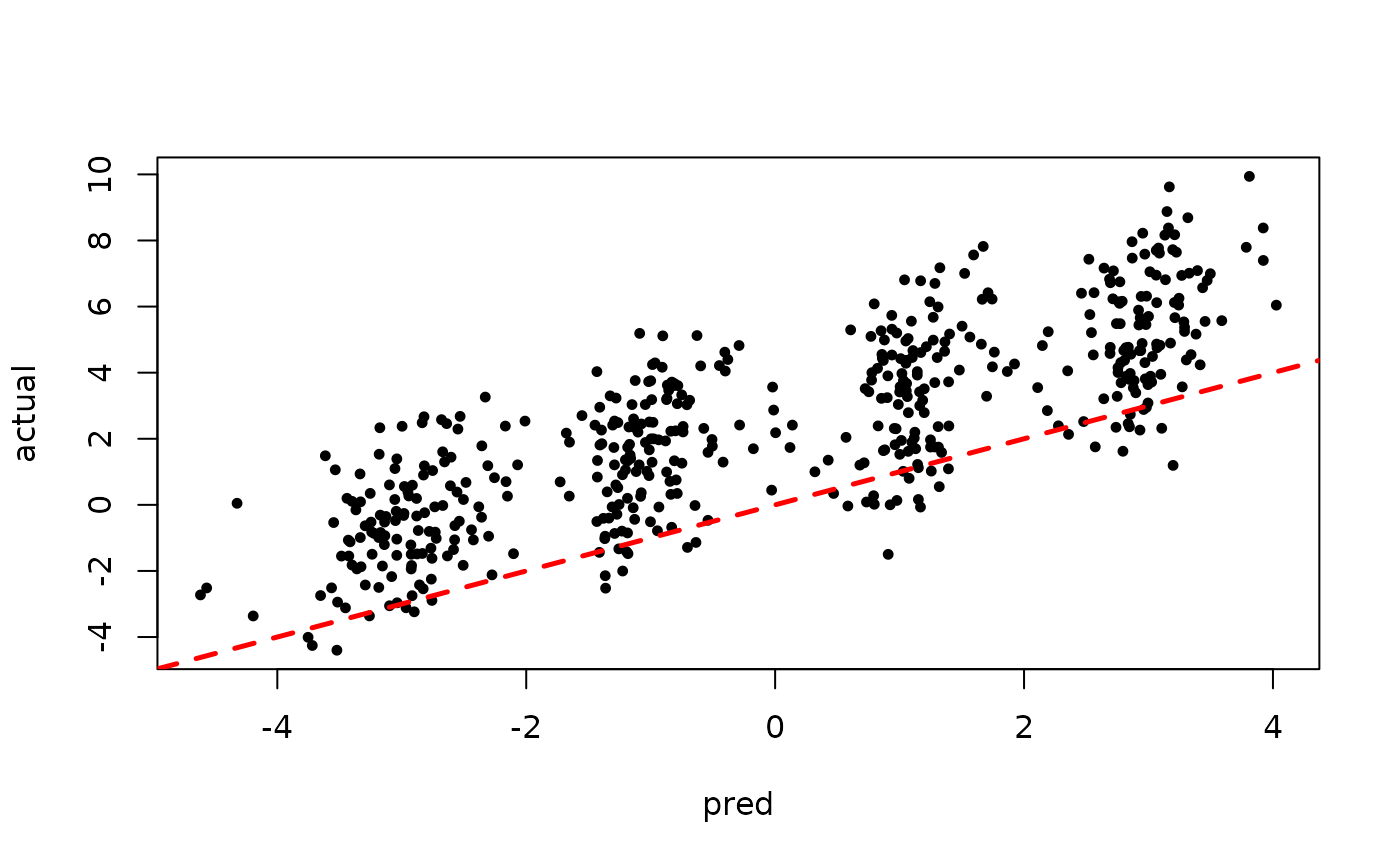

Demo 5: Causal Inference

Here we show how to implement the Bayesian Causal Forest (BCF) model of Hahn, Murray, and Carvalho (2020) using stochtree’s prototype API, including demoing a non-trivial sampling step done at the R level.

Background

While the supervised learning case of the previous demo is conceptually simple, we motivate the causal effect estimation task with some additional notation. Let $y$ refer to a continuous outcome of interest, $Z$ refer to a binary treatment, and $X$ to a set of covariates that may influence $Y$, $Z$, or both.

If $X$ is an exhaustive set of covariates that influence $Z$ and $Y$, we can specific $Y$ in terms of a causal model (see for example Pearl (2009)) as $$\begin{equation*} \begin{aligned} Y &= F(Z, X, \epsilon_Y) \end{aligned} \end{equation*}$$ where $\epsilon_Y$ is outcome specific random noise and $F$ is a function that generates $Y$ (in many cases, $F$ can be thought of as the inverse of the CDF conditional on $X$ and $Z$).

The “potential outcomes” (see Imbens and Rubin (2015)) can be recovered by $Y^1 = F(1, X, \epsilon_Y)$ and $Y^0 = F(0, X, \epsilon_Y)$.

The causal outcome model can be decomposed into “mean” and “error” terms as below $$\begin{equation*} \begin{aligned} Y &= \mu(X) + Z\tau(X) + \left[\eta(X) + Z\delta(X)\right]\\ \mu(X) &= \mathbb{E}_{\epsilon_Y}\left[F(0, X, \epsilon_Y)\right]\\ \tau(X) &= \mathbb{E}_{\epsilon_Y}\left[F(1, X, \epsilon_Y) - F(0, X, \epsilon_Y)\right]\\ \eta(X) &= F(0, X, \epsilon_Y) - \mathbb{E}_{\epsilon_Y}\left[F(0, X, \epsilon_Y)\right]\\ \delta(X) &= F(1, X, \epsilon_Y) - F(0, X, \epsilon_Y) - \mathbb{E}_{\epsilon_Y}\left[F(1, X, \epsilon_Y) - F(0, X, \epsilon_Y)\right] \end{aligned} \end{equation*}$$

Here $\tau(X)$ is precisely the conditional average treatment effect (CATE) estimand. Unfortunately, the functional form of $F$ is unavailable for analysis, so that $\tau(X)$ cannot be derived.

This is where flexible, regularized nonparametrics enter the picture, as we aim to estimate $\mu(X)$ and $\tau(X)$ from data.

Bayesian Causal Forest (BCF)

BCF estimates $\mu(X)$ and $\tau(X)$ using separate BART forests for each term. Furthermore, rather than rely on the common implicit coding of $Z$ as 0 for control observations and 1 for treated observations, they consider coding control observations with a parameter $b_0$ and treated observations with a parameter $b_1$. Placing a $N(0,1/2)$ prior on each $b_z$, this essentially redefines the outcome model as $$\begin{equation*} \begin{aligned} y &= \mu(X) + \tau(X) f(Z) + \epsilon\\ f(Z) &= b_0(1-Z) + b_1 Z\\ \epsilon &\sim N\left(0, \sigma^2\right)\\ b_0, b_1 &\sim N\left(0, 1/2\right) \end{aligned} \end{equation*}$$

Updating each $b_z$ requires an additional Gibbs step, which we derive here. Conditioning on sampled forests $\mu$ and $\tau$, we are essentially regressing $y - \mu(Z)$ on $\left[(1-Z)\tau(X), Z\tau(X)\right]$ which has a closed form posterior $$\begin{equation*} \begin{aligned} b_0 \mid y, X, \mu,\tau &\sim N\left(\frac{s_{y\tau,0}}{s_{\tau\tau,0} + 2\sigma^2}, \frac{\sigma^2}{s_{\tau\tau,0} + 2\sigma^2}\right)\\ b_1 \mid y, X, \mu,\tau &\sim N\left(\frac{s_{y\tau,1}}{s_{\tau\tau,1} + 2\sigma^2}, \frac{\sigma^2}{s_{\tau\tau,1} + 2\sigma^2}\right) \end{aligned} \end{equation*}$$ where $s_{y\tau,z} = \sum_{i: Z_i = z} (y_i - \mu(X_i))\tau(X_i)$ and $s_{\tau\tau,z} = \sum_{i: Z_i = z} \tau(X_i)\tau(X_i)$.

Simulation

The simulated causal DGP mirrors the nonlinear, heterogeneous treatment effect DGP presented in Hahn, Murray, and Carvalho (2020).

n <- 500
x1 <- rnorm(n)
x2 <- rnorm(n)
x3 <- rnorm(n)
x4 <- as.numeric(rbinom(n,1,0.5))
x5 <- as.numeric(sample(1:3,n,replace=TRUE))
X <- cbind(x1,x2,x3,x4,x5)
p <- ncol(X)
g <- function(x) {ifelse(x[,5]==1,2,ifelse(x[,5]==2,-1,4))}
mu1 <- function(x) {1+g(x)+x[,1]*x[,3]}
mu2 <- function(x) {1+g(x)+6*abs(x[,3]-1)}
tau1 <- function(x) {rep(3,nrow(x))}
tau2 <- function(x) {1+2*x[,2]*x[,4]}
mu_x <- mu1(X)
tau_x <- tau2(X)
pi_x <- 0.8*pnorm((3*mu_x/sd(mu_x)) - 0.5*X[,1]) + 0.05 + runif(n)/10
Z <- rbinom(n,1,pi_x)
E_XZ <- mu_x + Z*tau_x
snr <- 4
y <- E_XZ + rnorm(n, 0, 1)*(sd(E_XZ)/snr)

# Standardize outcome
y_bar <- mean(y)
y_std <- sd(y)
resid <- (y-y_bar)/y_std

Sampling

Set some parameters that inform the forest and variance parameter samplers

# Mu forest
alpha_mu <- 0.95
beta_mu <- 2.0
min_samples_leaf_mu <- 5
max_depth_mu <- 10
num_trees_mu <- 250
cutpoint_grid_size_mu = 100
tau_init_mu = 1/num_trees_mu
leaf_prior_scale_mu = matrix(c(tau_init_mu), ncol = 1)
a_leaf_mu <- 3.
b_leaf_mu <- var(resid)/(num_trees_mu)
leaf_regression_mu <- F
sigma_leaf_mu <- var(resid)/(num_trees_mu)
current_leaf_scale_mu <- as.matrix(sigma_leaf_mu)

# Tau forest
alpha_tau <- 0.25
beta_tau <- 3.0
min_samples_leaf_tau <- 5
max_depth_tau <- 10
num_trees_tau <- 50
cutpoint_grid_size_tau = 100
a_leaf_tau <- 3.
b_leaf_tau <- var(resid)/(2*num_trees_tau)
leaf_regression_tau <- T
sigma_leaf_tau <- var(resid)/(2*num_trees_tau)
current_leaf_scale_tau <- as.matrix(sigma_leaf_tau)

# Common parameters
nu <- 3
sigma2hat <- (sigma(lm(resid~X)))^2
quantile_cutoff <- 0.9
if (is.null(lambda)) {
    lambda <- (sigma2hat*qgamma(1-quantile_cutoff,nu))/nu
}
sigma2 <- sigma2hat
current_sigma2 <- sigma2

Prepare to run the sampler (now we must specify initial values for $b_0$ and $b_1$, for which we choose -1/2 and 1/2 instead of 0 and 1).

# Sampling composition
num_gfr <- 20
num_burnin <- 0
num_mcmc <- 100
num_samples <- num_gfr + num_burnin + num_mcmc

# Sigma^2 samples
global_var_samples <- rep(0, num_samples)

# Adaptive coding parameter samples
b_0_samples <- rep(0, num_samples)
b_1_samples <- rep(0, num_samples)
b_0 <- -0.5
b_1 <- 0.5
current_b_0 <- b_0
current_b_1 <- b_1
tau_basis <- (1-Z)*current_b_0 + Z*current_b_1

Initialize R-level access to the C++ classes needed to sample our model

# Data
X_mu <- cbind(X, pi_x)
X_tau <- X
feature_types <- c(0,0,0,1,1)
feature_types_mu <- as.integer(c(feature_types,0))
feature_types_tau <- as.integer(feature_types)
variable_weights_mu = rep(1/ncol(X_mu), ncol(X_mu))
variable_weights_tau = rep(1/ncol(X_tau), ncol(X_tau))
forest_dataset_mu <- createForestDataset(X_mu)
forest_dataset_tau <- createForestDataset(X_tau, tau_basis)
outcome <- createOutcome(resid)

# Random number generator (std::mt19937)
rng <- createRNG()

# Sampling data structures
forest_model_mu <- createForestModel(
    forest_dataset_mu, feature_types_mu, num_trees_mu, nrow(X_mu), 
    alpha_mu, beta_mu, min_samples_leaf_mu, max_depth_mu
)
forest_model_tau <- createForestModel(
    forest_dataset_tau, feature_types_tau, num_trees_tau, nrow(X_tau), 
    alpha_tau, beta_tau, min_samples_leaf_tau, max_depth_tau
)

# Container of forest samples
forest_samples_mu <- createForestContainer(num_trees_mu, 1, T)
active_forest_mu <- createForest(num_trees_mu, 1, T)
forest_samples_tau <- createForestContainer(num_trees_tau, 1, F)
active_forest_tau <- createForest(num_trees_tau, 1, F)

# Initialize the leaves of each tree in the prognostic forest
active_forest_mu$prepare_for_sampler(forest_dataset_mu, outcome, forest_model_mu, 0, mean(resid))
active_forest_mu$adjust_residual(forest_dataset_mu, outcome, forest_model_mu, F, F)

# Initialize the leaves of each tree in the treatment effect forest
active_forest_tau$prepare_for_sampler(forest_dataset_tau, outcome, forest_model_tau, 1, 0.)
active_forest_tau$adjust_residual(forest_dataset_tau, outcome, forest_model_tau, T, F)

Run the grow-from-root sampler to “warm-start” BART, also updating the adaptive coding parameter $b_0$ and $b_1$

if (num_gfr > 0){
    for (i in 1:num_gfr) {
        # Sample the prognostic forest
        forest_model_mu$sample_one_iteration(
            forest_dataset_mu, outcome, forest_samples_mu, active_forest_mu, rng, 
            feature_types_mu, 0, current_leaf_scale_mu, variable_weights_mu, 
            1, 1, current_sigma2, cutpoint_grid_size, keep_forest = T, gfr = T, 
            pre_initialized = T
        )
        
        # Sample variance parameters (if requested)
        global_var_samples[i] <- sample_sigma2_one_iteration(
            outcome, forest_dataset_mu, rng, nu, lambda
        )
        current_sigma2 <- global_var_samples[i]

        # Sample the treatment forest
        forest_model_tau$sample_one_iteration(
            forest_dataset_tau, outcome, forest_samples_tau, active_forest_tau, rng, 
            feature_types_tau, 1, current_leaf_scale_tau, variable_weights_tau, 
            1, 1, current_sigma2, cutpoint_grid_size, keep_forest = T, gfr = T, 
            pre_initialized = T
        )
        
        # Sample adaptive coding parameters
        mu_x_raw <- active_forest_mu$predict_raw(forest_dataset_mu)
        tau_x_raw <- active_forest_tau$predict_raw(forest_dataset_tau)
        s_tt0 <- sum(tau_x_raw*tau_x_raw*(Z==0))
        s_tt1 <- sum(tau_x_raw*tau_x_raw*(Z==1))
        partial_resid_mu <- resid - mu_x_raw
        s_ty0 <- sum(tau_x_raw*partial_resid_mu*(Z==0))
        s_ty1 <- sum(tau_x_raw*partial_resid_mu*(Z==1))
        current_b_0 <- rnorm(1, (s_ty0/(s_tt0 + 2*current_sigma2)), 
                             sqrt(current_sigma2/(s_tt0 + 2*current_sigma2)))
        current_b_1 <- rnorm(1, (s_ty1/(s_tt1 + 2*current_sigma2)), 
                             sqrt(current_sigma2/(s_tt1 + 2*current_sigma2)))
        tau_basis <- (1-Z)*current_b_0 + Z*current_b_1
        forest_dataset_tau$update_basis(tau_basis)
        forest_model_tau$propagate_basis_update(forest_dataset_tau, outcome, active_forest_tau)
        b_0_samples[i] <- current_b_0
        b_1_samples[i] <- current_b_1
        
        # Sample variance parameters (if requested)
        global_var_samples[i] <- sample_sigma2_one_iteration(outcome, forest_dataset_tau, rng, nu, lambda)
        current_sigma2 <- global_var_samples[i]
    }
}

Pick up from the last GFR forest (and associated global variance / leaf scale parameters) with an MCMC sampler

if (num_burnin + num_mcmc > 0) {
    for (i in (num_gfr+1):num_samples) {
        # Sample the prognostic forest
        forest_model_mu$sample_one_iteration(
            forest_dataset_mu, outcome, forest_samples_mu, active_forest_mu, rng, feature_types_mu, 
            0, current_leaf_scale_mu, variable_weights_mu, 1, 1, current_sigma2, 
            cutpoint_grid_size, keep_forest = T, gfr = F, pre_initialized = T
        )
        
        # Sample global variance parameter
        global_var_samples[i] <- sample_sigma2_one_iteration(outcome, forest_dataset_mu, rng, nu, lambda)
        current_sigma2 <- global_var_samples[i]

        # Sample the treatment forest
        forest_model_tau$sample_one_iteration(
            forest_dataset_tau, outcome, forest_samples_tau, active_forest_tau, rng, feature_types_tau, 
            1, current_leaf_scale_tau, variable_weights_tau, 1, 1, current_sigma2, 
            cutpoint_grid_size, keep_forest = T, gfr = F, pre_initialized = T
        )
        
        # Sample coding parameters
        mu_x_raw <- active_forest_mu$predict_raw(forest_dataset_mu)
        tau_x_raw <- active_forest_tau$predict_raw(forest_dataset_tau)
        s_tt0 <- sum(tau_x_raw*tau_x_raw*(Z==0))
        s_tt1 <- sum(tau_x_raw*tau_x_raw*(Z==1))
        partial_resid_mu <- resid - mu_x_raw
        s_ty0 <- sum(tau_x_raw*partial_resid_mu*(Z==0))
        s_ty1 <- sum(tau_x_raw*partial_resid_mu*(Z==1))
        current_b_0 <- rnorm(1, (s_ty0/(s_tt0 + 2*current_sigma2)), 
                             sqrt(current_sigma2/(s_tt0 + 2*current_sigma2)))
        current_b_1 <- rnorm(1, (s_ty1/(s_tt1 + 2*current_sigma2)), 
                             sqrt(current_sigma2/(s_tt1 + 2*current_sigma2)))
        tau_basis <- (1-Z)*current_b_0 + Z*current_b_1
        forest_dataset_tau$update_basis(tau_basis)
        forest_model_tau$propagate_basis_update(forest_dataset_tau, outcome, active_forest_tau)
        b_0_samples[i] <- current_b_0
        b_1_samples[i] <- current_b_1

        # Sample global variance parameter
        global_var_samples[i] <- sample_sigma2_one_iteration(outcome, forest_dataset_tau, rng, nu, lambda)
        current_sigma2 <- global_var_samples[i]
    }
}

Predict and rescale samples

# Forest predictions
mu_hat <- forest_samples_mu$predict(forest_dataset_mu)*y_std + y_bar
tau_hat_raw <- forest_samples_tau$predict_raw(forest_dataset_tau)
tau_hat <- t(t(tau_hat_raw) * (b_1_samples - b_0_samples))*y_std
y_hat <- mu_hat + tau_hat * as.numeric(Z)

# Global error variance
sigma2_samples <- global_var_samples*(y_std^2)

Results

Inspect the XBART results

plot(sigma2_samples[1:num_gfr], ylab="sigma^2")

plot(rowMeans(mu_hat[,1:num_gfr]), mu_x, pch=16, cex=0.75, 
     xlab = "pred", ylab = "actual", main = "prognostic term")
abline(0,1,col="red",lty=2,lwd=2.5)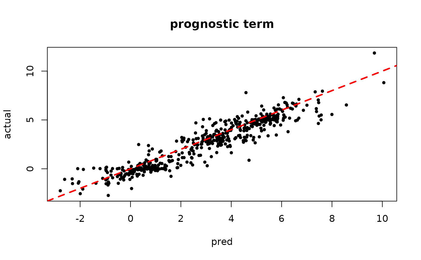

plot(rowMeans(tau_hat[,1:num_gfr]), tau_x, pch=16, cex=0.75, 
     xlab = "pred", ylab = "actual", main = "treatment effect term")
abline(0,1,col="red",lty=2,lwd=2.5)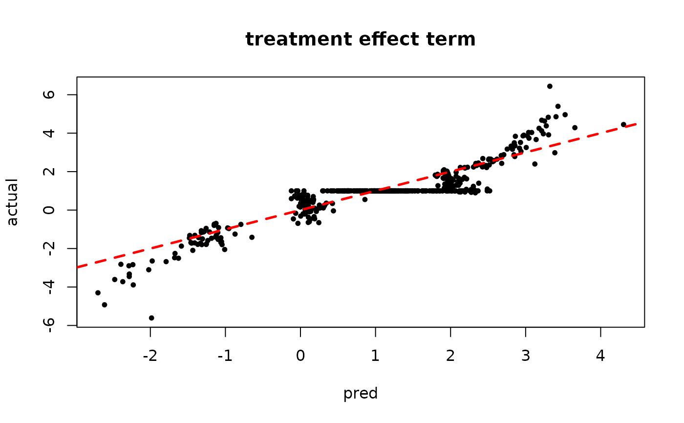

mean((rowMeans(tau_hat[,1:num_gfr]) - tau_x)^2)
#> [1] 0.264747

Inspect the warm start BART results

plot(sigma2_samples[(num_gfr+1):num_samples], ylab="sigma^2")

plot(rowMeans(mu_hat[,(num_gfr+1):num_samples]), mu_x, pch=16, cex=0.75, 
     xlab = "pred", ylab = "actual", main = "prognostic term")
abline(0,1,col="red",lty=2,lwd=2.5)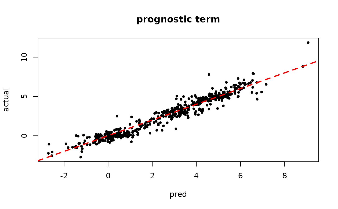

plot(rowMeans(tau_hat[,(num_gfr+1):num_samples]), tau_x, pch=16, cex=0.75, 
     xlab = "pred", ylab = "actual", main = "treatment effect term")
abline(0,1,col="red",lty=2,lwd=2.5)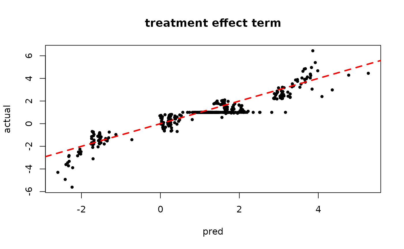

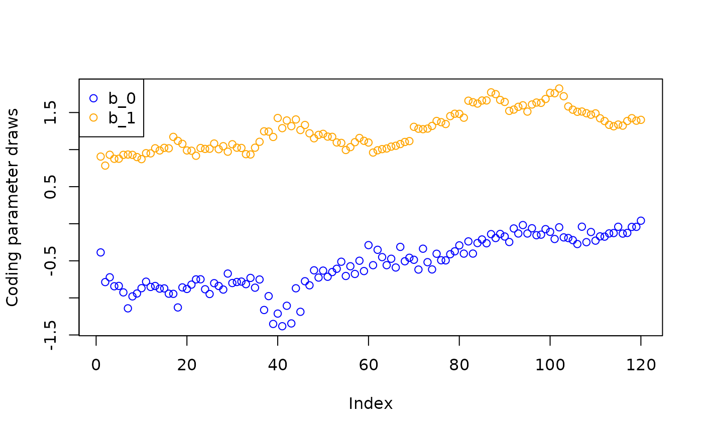
mean((rowMeans(tau_hat[,(num_gfr+1):num_samples]) - tau_x)^2)
#> [1] 0.320933

Inspect the “adaptive coding” parameters $b_0$ and $b_1$.

plot(b_0_samples, col = "blue", ylab = "Coding parameter draws", 
     ylim = c(min(min(b_0_samples), min(b_1_samples)), max(max(b_0_samples), max(b_1_samples))))
points(b_1_samples, col = "orange")
legend("topleft", legend = c("b_0", "b_1"), col = c("blue", "orange"), pch = c(1,1))

References

Hahn, P Richard, Jared S Murray, and Carlos M Carvalho. 2020. “Bayesian Regression Tree Models for Causal Inference: Regularization, Confounding, and Heterogeneous Effects (with Discussion).” Bayesian Analysis 15 (3): 965–1056.

He, Jingyu, and P Richard Hahn. 2023. “Stochastic Tree Ensembles for Regularized Nonlinear Regression.” Journal of the American Statistical Association 118 (541): 551–70.

Imbens, Guido W, and Donald B Rubin. 2015. Causal Inference in Statistics, Social, and Biomedical Sciences. Cambridge university press.

Murray, Jared S. 2021. “Log-Linear Bayesian Additive Regression Trees for Multinomial Logistic and Count Regression Models.” Journal of the American Statistical Association 116 (534): 756–69.

Pearl, Judea. 2009. Causality. Cambridge university press.

Pratola, Matthew T, Hugh A Chipman, Edward I George, and Robert E McCulloch. 2020. “Heteroscedastic BART via Multiplicative Regression Trees.” Journal of Computational and Graphical Statistics 29 (2): 405–17.