Causal Machine Learning in StochTree
CausalInference.RmdThis vignette demonstrates how to use the bcf() function
for supervised learning. To begin, we load the stochtree package.
We also define several simple functions that configure the data generating processes used in this vignette.
g <- function(x) {ifelse(x[,5]==1,2,ifelse(x[,5]==2,-1,-4))}
mu1 <- function(x) {1+g(x)+x[,1]*x[,3]}
mu2 <- function(x) {1+g(x)+6*abs(x[,3]-1)}
tau1 <- function(x) {rep(3,nrow(x))}
tau2 <- function(x) {1+2*x[,2]*x[,4]}
Binary Treatment
Demo 1: Nonlinear Outcome Model, Heterogeneous Treatment Effect
We consider the following data generating process from Hahn, Murray, and Carvalho (2020):
Simulation
We draw from the DGP defined above
n <- 500
snr <- 3
x1 <- rnorm(n)
x2 <- rnorm(n)
x3 <- rnorm(n)
x4 <- as.numeric(rbinom(n,1,0.5))
x5 <- as.numeric(sample(1:3,n,replace=TRUE))
X <- cbind(x1,x2,x3,x4,x5)
p <- ncol(X)
mu_x <- mu1(X)
tau_x <- tau2(X)
pi_x <- 0.8*pnorm((3*mu_x/sd(mu_x)) - 0.5*X[,1]) + 0.05 + runif(n)/10
Z <- rbinom(n,1,pi_x)
E_XZ <- mu_x + Z*tau_x
y <- E_XZ + rnorm(n, 0, 1)*(sd(E_XZ)/snr)
X <- as.data.frame(X)
X$x4 <- factor(X$x4, ordered = TRUE)
X$x5 <- factor(X$x5, ordered = TRUE)

# Split data into test and train sets
test_set_pct <- 0.2
n_test <- round(test_set_pct*n)
n_train <- n - n_test
test_inds <- sort(sample(1:n, n_test, replace = FALSE))
train_inds <- (1:n)[!((1:n) %in% test_inds)]
X_test <- X[test_inds,]
X_train <- X[train_inds,]
pi_test <- pi_x[test_inds]
pi_train <- pi_x[train_inds]
Z_test <- Z[test_inds]
Z_train <- Z[train_inds]
y_test <- y[test_inds]
y_train <- y[train_inds]
mu_test <- mu_x[test_inds]
mu_train <- mu_x[train_inds]
tau_test <- tau_x[test_inds]
tau_train <- tau_x[train_inds]
Sampling and Analysis
Warmstart
We first simulate from an ensemble model of
using “warm-start” initialization samples (Krantsevich, He, and Hahn (2023)). This is the
default in stochtree.
num_gfr <- 10
num_burnin <- 0
num_mcmc <- 1000
num_samples <- num_gfr + num_burnin + num_mcmc
bcf_params <- list(sample_sigma_leaf_mu = F, sample_sigma_leaf_tau = F,
                   keep_every = 5)
bcf_model_warmstart <- bcf(
    X_train = X_train, Z_train = Z_train, y_train = y_train, pi_train = pi_train,
    X_test = X_test, Z_test = Z_test, pi_test = pi_test,
    num_gfr = num_gfr, num_burnin = num_burnin, num_mcmc = num_mcmc,
    params = bcf_params
)
#> Warning in t(tau_hat_train_raw) * (b_1_samples - b_0_samples): longer object
#> length is not a multiple of shorter object length
#> Warning in t(tau_hat_test_raw) * (b_1_samples - b_0_samples): longer object
#> length is not a multiple of shorter object length
Inspect the BART samples that were initialized with an XBART warm-start
plot(rowMeans(bcf_model_warmstart$mu_hat_test), mu_test,
     xlab = "predicted", ylab = "actual", main = "Prognostic function")
abline(0,1,col="red",lty=3,lwd=3)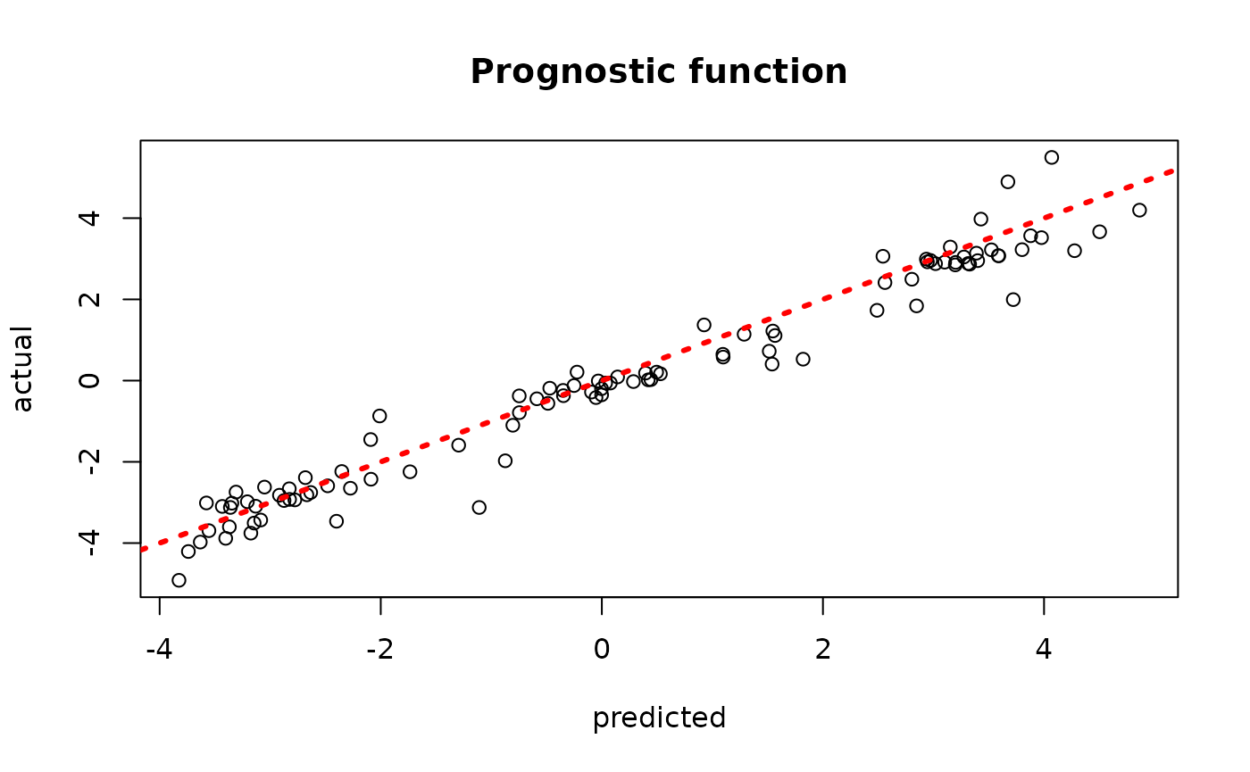
plot(rowMeans(bcf_model_warmstart$tau_hat_test), tau_test,
     xlab = "predicted", ylab = "actual", main = "Treatment effect")
abline(0,1,col="red",lty=3,lwd=3)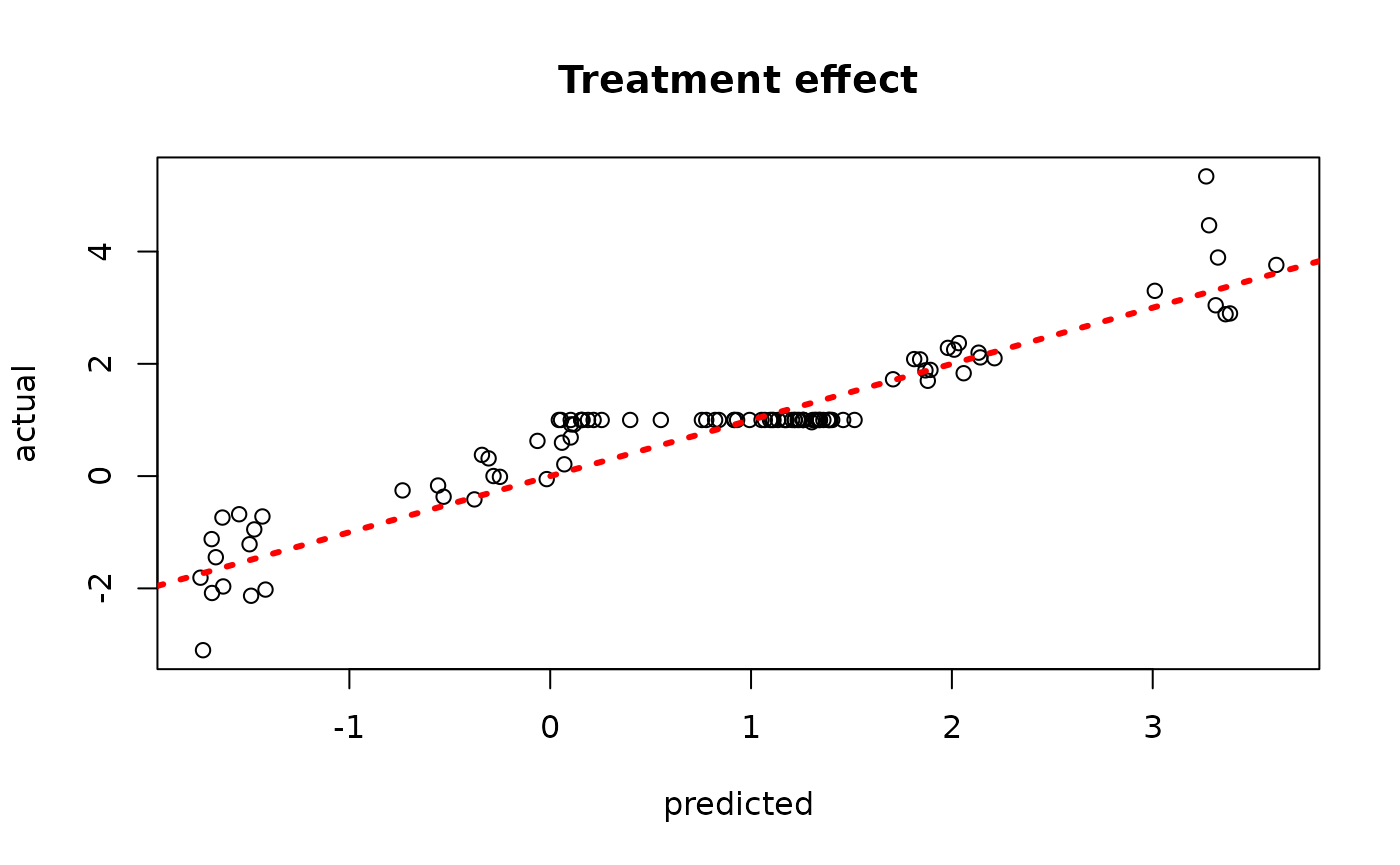
sigma_observed <- var(y-E_XZ)
plot_bounds <- c(min(c(bcf_model_warmstart$sigma2_samples, sigma_observed)),
                 max(c(bcf_model_warmstart$sigma2_samples, sigma_observed)))
plot(bcf_model_warmstart$sigma2_samples, ylim = plot_bounds,
     ylab = "sigma^2", xlab = "Sample", main = "Global variance parameter")
abline(h = sigma_observed, lty=3, lwd = 3, col = "blue")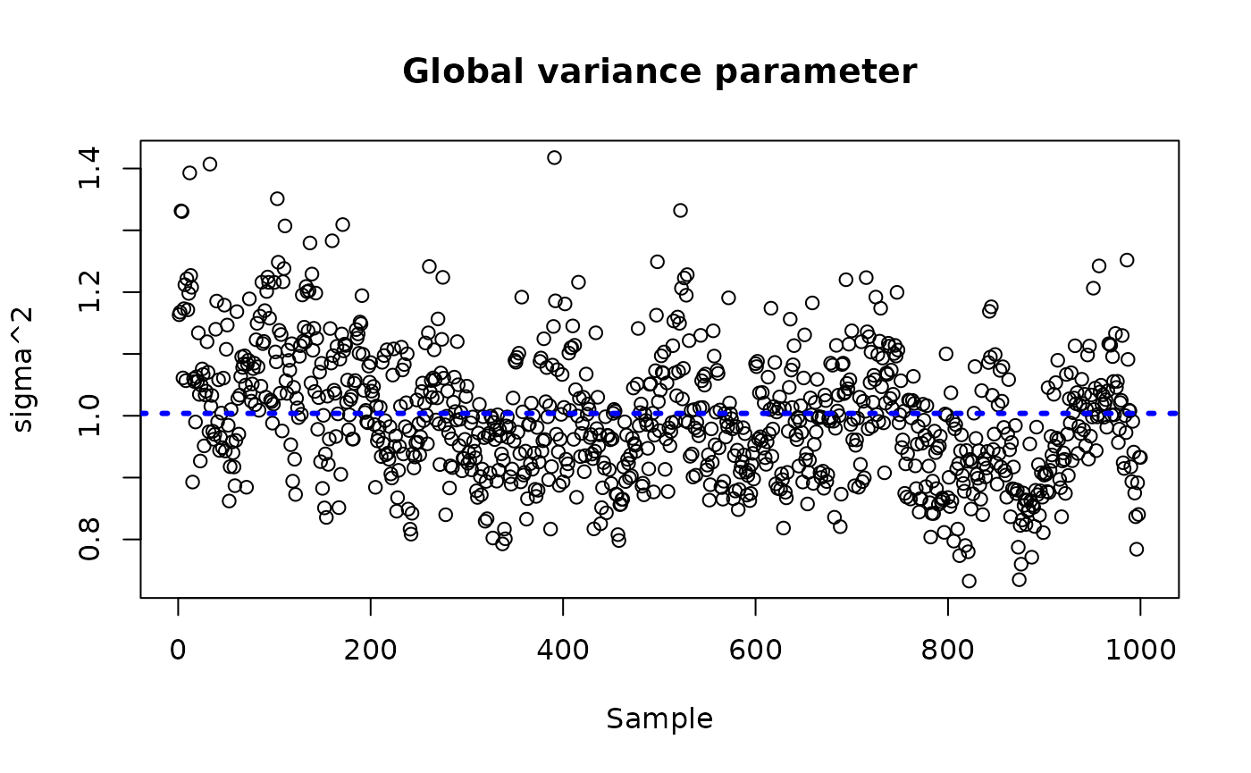
Examine test set interval coverage
BART MCMC without Warmstart
Next, we simulate from this ensemble model without any warm-start initialization.
num_gfr <- 0
num_burnin <- 1000
num_mcmc <- 1000
num_samples <- num_gfr + num_burnin + num_mcmc
bcf_params <- list(sample_sigma_leaf_mu = F, sample_sigma_leaf_tau = F,
                   keep_every = 5)
bcf_model_root <- bcf(
    X_train = X_train, Z_train = Z_train, y_train = y_train, pi_train = pi_train,
    X_test = X_test, Z_test = Z_test, pi_test = pi_test,
    num_gfr = num_gfr, num_burnin = num_burnin, num_mcmc = num_mcmc,
    params = bcf_params
)
Inspect the BART samples after burnin
plot(rowMeans(bcf_model_root$mu_hat_test), mu_test,
     xlab = "predicted", ylab = "actual", main = "Prognostic function")
abline(0,1,col="red",lty=3,lwd=3)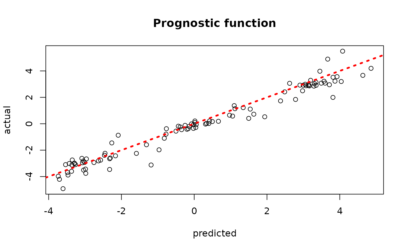
plot(rowMeans(bcf_model_root$tau_hat_test), tau_test,
     xlab = "predicted", ylab = "actual", main = "Treatment effect")
abline(0,1,col="red",lty=3,lwd=3)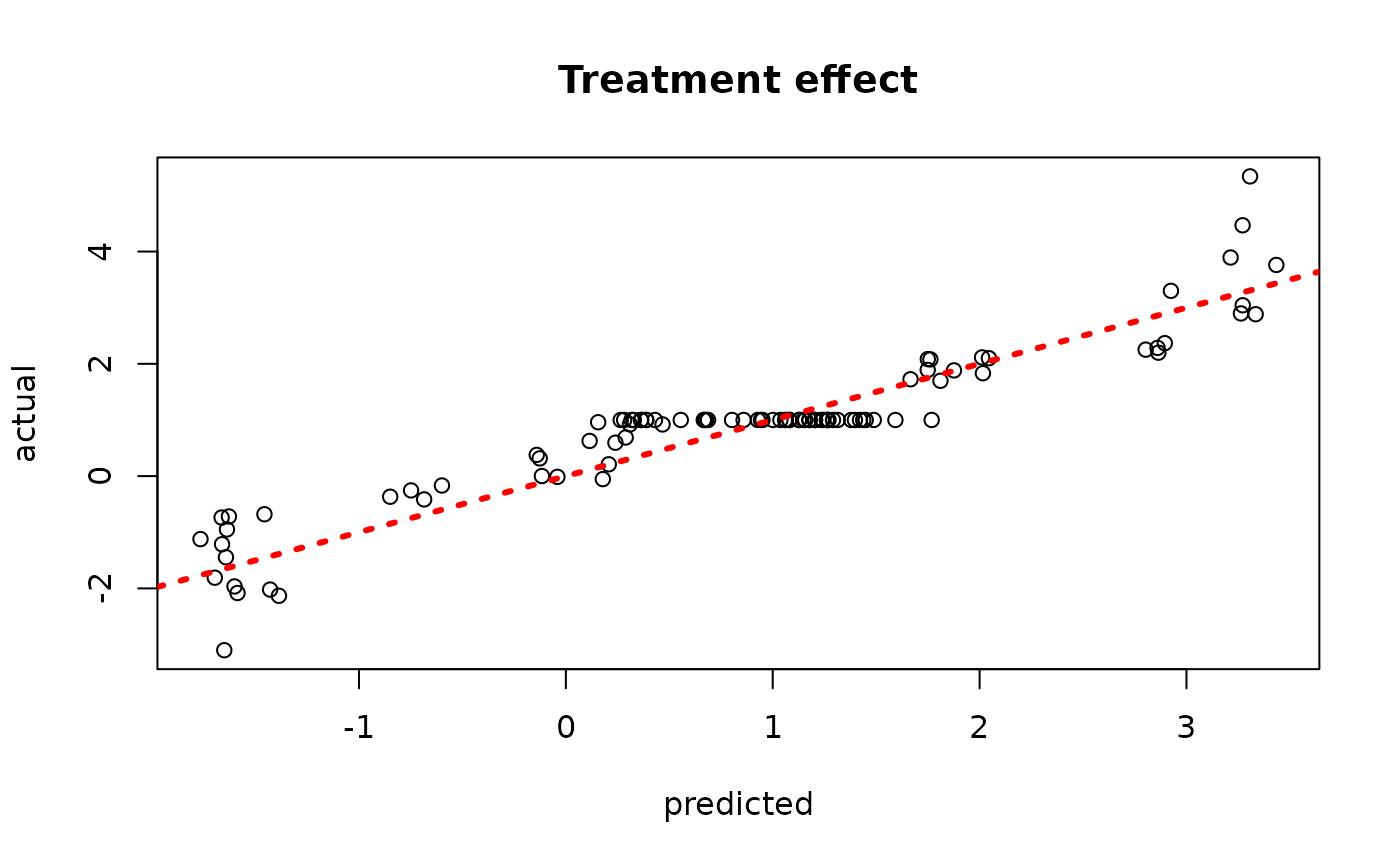
sigma_observed <- var(y-E_XZ)
plot_bounds <- c(min(c(bcf_model_root$sigma2_samples, sigma_observed)),
                 max(c(bcf_model_root$sigma2_samples, sigma_observed)))
plot(bcf_model_root$sigma2_samples, ylim = plot_bounds,
     ylab = "sigma^2", xlab = "Sample", main = "Global variance parameter")
abline(h = sigma_observed, lty=3, lwd = 3, col = "blue")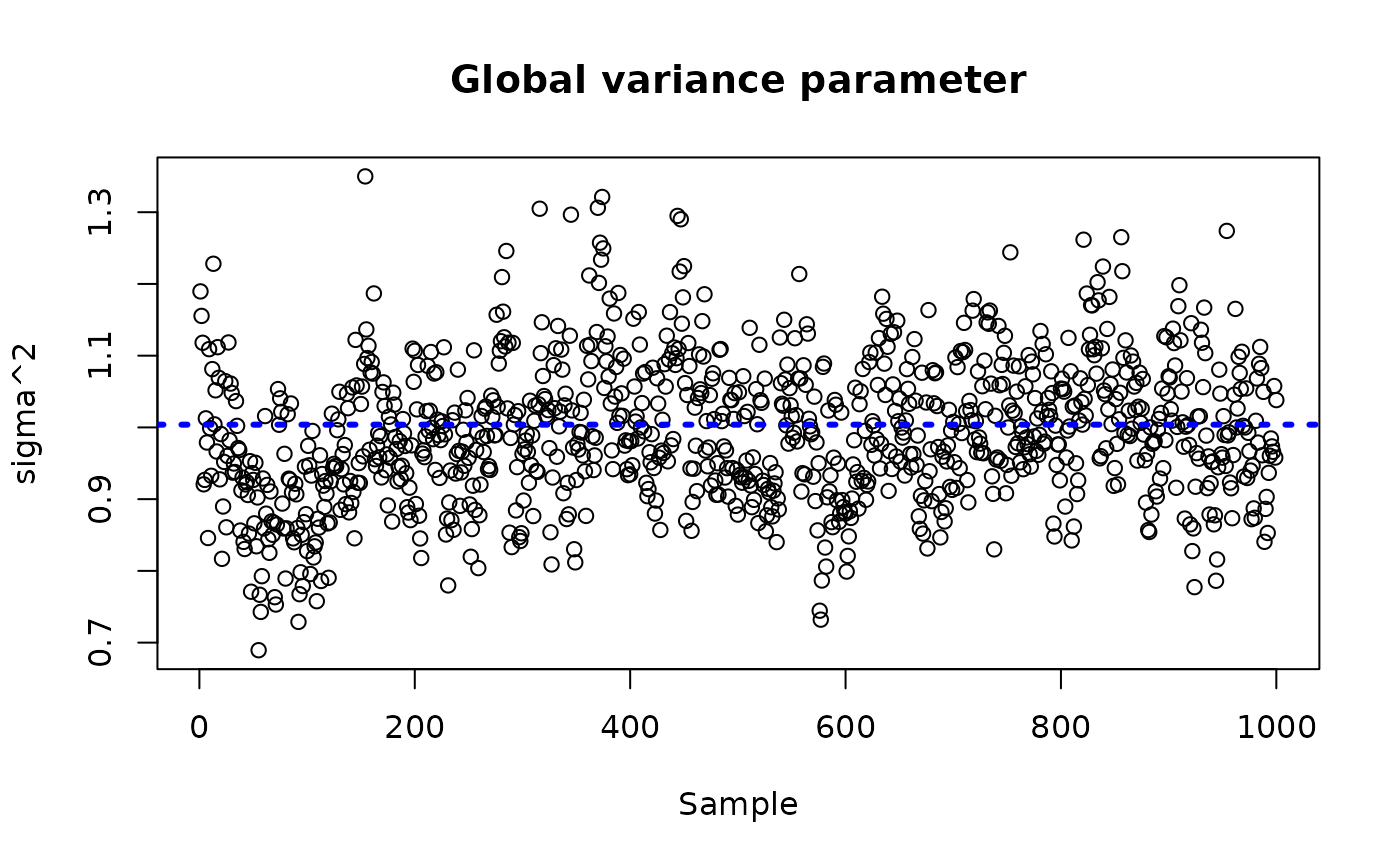
Examine test set interval coverage
Demo 2: Linear Outcome Model, Heterogeneous Treatment Effect
We consider the following data generating process from Hahn, Murray, and Carvalho (2020):
Simulation
We draw from the DGP defined above
n <- 500
snr <- 3
x1 <- rnorm(n)
x2 <- rnorm(n)
x3 <- rnorm(n)
x4 <- as.numeric(rbinom(n,1,0.5))
x5 <- as.numeric(sample(1:3,n,replace=TRUE))
X <- cbind(x1,x2,x3,x4,x5)
p <- ncol(X)
mu_x <- mu2(X)
tau_x <- tau2(X)
pi_x <- 0.8*pnorm((3*mu_x/sd(mu_x)) - 0.5*X[,1]) + 0.05 + runif(n)/10
Z <- rbinom(n,1,pi_x)
E_XZ <- mu_x + Z*tau_x
y <- E_XZ + rnorm(n, 0, 1)*(sd(E_XZ)/snr)
X <- as.data.frame(X)
X$x4 <- factor(X$x4, ordered = TRUE)
X$x5 <- factor(X$x5, ordered = TRUE)

# Split data into test and train sets
test_set_pct <- 0.2
n_test <- round(test_set_pct*n)
n_train <- n - n_test
test_inds <- sort(sample(1:n, n_test, replace = FALSE))
train_inds <- (1:n)[!((1:n) %in% test_inds)]
X_test <- X[test_inds,]
X_train <- X[train_inds,]
pi_test <- pi_x[test_inds]
pi_train <- pi_x[train_inds]
Z_test <- Z[test_inds]
Z_train <- Z[train_inds]
y_test <- y[test_inds]
y_train <- y[train_inds]
mu_test <- mu_x[test_inds]
mu_train <- mu_x[train_inds]
tau_test <- tau_x[test_inds]
tau_train <- tau_x[train_inds]
Sampling and Analysis
Warmstart
We first simulate from an ensemble model of
using “warm-start” initialization samples (Krantsevich, He, and Hahn (2023)). This is the
default in stochtree.
num_gfr <- 10
num_burnin <- 0
num_mcmc <- 100
num_samples <- num_gfr + num_burnin + num_mcmc
bcf_params <- list(sample_sigma_leaf_mu = F, sample_sigma_leaf_tau = F,
                   keep_every = 5)
bcf_model_warmstart <- bcf(
    X_train = X_train, Z_train = Z_train, y_train = y_train, pi_train = pi_train,
    X_test = X_test, Z_test = Z_test, pi_test = pi_test,
    num_gfr = num_gfr, num_burnin = num_burnin, num_mcmc = num_mcmc,
    params = bcf_params
)
#> Warning in t(tau_hat_train_raw) * (b_1_samples - b_0_samples): longer object
#> length is not a multiple of shorter object length
#> Warning in t(tau_hat_test_raw) * (b_1_samples - b_0_samples): longer object
#> length is not a multiple of shorter object length
Inspect the BART samples that were initialized with an XBART warm-start
plot(rowMeans(bcf_model_warmstart$mu_hat_test), mu_test,
     xlab = "predicted", ylab = "actual", main = "Prognostic function")
abline(0,1,col="red",lty=3,lwd=3)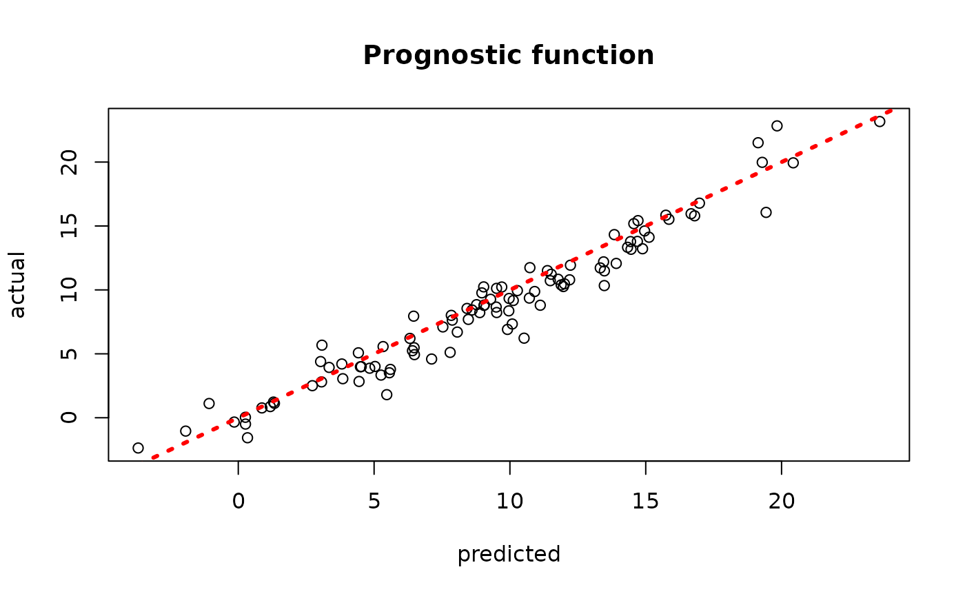
plot(rowMeans(bcf_model_warmstart$tau_hat_test), tau_test,
     xlab = "predicted", ylab = "actual", main = "Treatment effect")
abline(0,1,col="red",lty=3,lwd=3)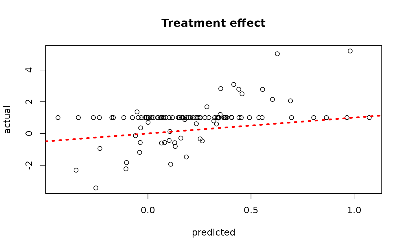
sigma_observed <- var(y-E_XZ)
plot_bounds <- c(min(c(bcf_model_warmstart$sigma2_samples, sigma_observed)),
                 max(c(bcf_model_warmstart$sigma2_samples, sigma_observed)))
plot(bcf_model_warmstart$sigma2_samples, ylim = plot_bounds,
     ylab = "sigma^2", xlab = "Sample", main = "Global variance parameter")
abline(h = sigma_observed, lty=3, lwd = 3, col = "blue")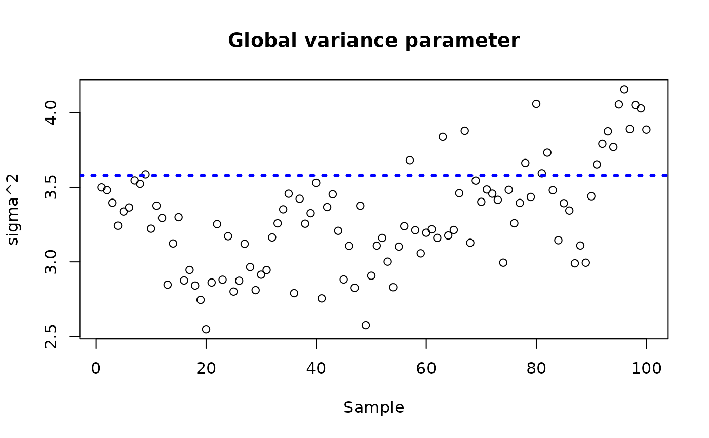
Examine test set interval coverage
BART MCMC without Warmstart
Next, we simulate from this ensemble model without any warm-start initialization.
num_gfr <- 0
num_burnin <- 100
num_mcmc <- 100
num_samples <- num_gfr + num_burnin + num_mcmc
bcf_params <- list(sample_sigma_leaf_mu = F, sample_sigma_leaf_tau = F,
                   keep_every = 5)
bcf_model_root <- bcf(
    X_train = X_train, Z_train = Z_train, y_train = y_train, pi_train = pi_train,
    X_test = X_test, Z_test = Z_test, pi_test = pi_test,
    num_gfr = num_gfr, num_burnin = num_burnin, num_mcmc = num_mcmc,
    params = bcf_params
)
Inspect the BART samples after burnin
plot(rowMeans(bcf_model_root$mu_hat_test), mu_test,
     xlab = "predicted", ylab = "actual", main = "Prognostic function")
abline(0,1,col="red",lty=3,lwd=3)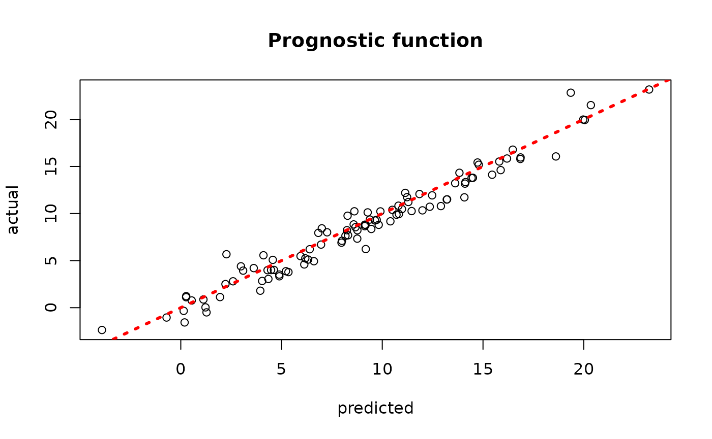
plot(rowMeans(bcf_model_root$tau_hat_test), tau_test,
     xlab = "predicted", ylab = "actual", main = "Treatment effect")
abline(0,1,col="red",lty=3,lwd=3)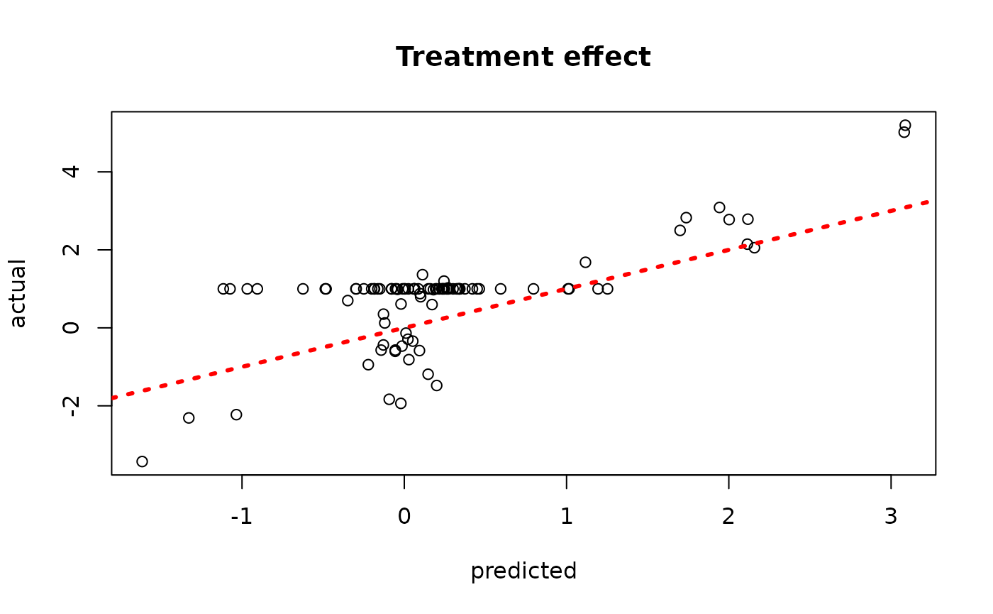
sigma_observed <- var(y-E_XZ)
plot_bounds <- c(min(c(bcf_model_root$sigma2_samples, sigma_observed)),
                 max(c(bcf_model_root$sigma2_samples, sigma_observed)))
plot(bcf_model_root$sigma2_samples, ylim = plot_bounds,
     ylab = "sigma^2", xlab = "Sample", main = "Global variance parameter")
abline(h = sigma_observed, lty=3, lwd = 3, col = "blue")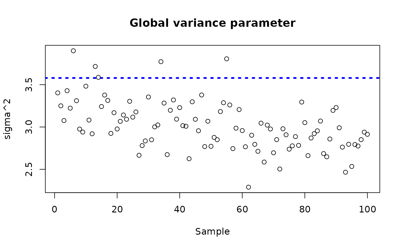
Examine test set interval coverage
Demo 3: Linear Outcome Model, Homogeneous Treatment Effect
We consider the following data generating process from Hahn, Murray, and Carvalho (2020):
Simulation
We draw from the DGP defined above
n <- 500
snr <- 3
x1 <- rnorm(n)
x2 <- rnorm(n)
x3 <- rnorm(n)
x4 <- as.numeric(rbinom(n,1,0.5))
x5 <- as.numeric(sample(1:3,n,replace=TRUE))
X <- cbind(x1,x2,x3,x4,x5)
p <- ncol(X)
mu_x <- mu2(X)
tau_x <- tau1(X)
pi_x <- 0.8*pnorm((3*mu_x/sd(mu_x)) - 0.5*X[,1]) + 0.05 + runif(n)/10
Z <- rbinom(n,1,pi_x)
E_XZ <- mu_x + Z*tau_x
y <- E_XZ + rnorm(n, 0, 1)*(sd(E_XZ)/snr)
X <- as.data.frame(X)
X$x4 <- factor(X$x4, ordered = TRUE)
X$x5 <- factor(X$x5, ordered = TRUE)

# Split data into test and train sets
test_set_pct <- 0.2
n_test <- round(test_set_pct*n)
n_train <- n - n_test
test_inds <- sort(sample(1:n, n_test, replace = FALSE))
train_inds <- (1:n)[!((1:n) %in% test_inds)]
X_test <- X[test_inds,]
X_train <- X[train_inds,]
pi_test <- pi_x[test_inds]
pi_train <- pi_x[train_inds]
Z_test <- Z[test_inds]
Z_train <- Z[train_inds]
y_test <- y[test_inds]
y_train <- y[train_inds]
mu_test <- mu_x[test_inds]
mu_train <- mu_x[train_inds]
tau_test <- tau_x[test_inds]
tau_train <- tau_x[train_inds]
Sampling and Analysis
Warmstart
We first simulate from an ensemble model of
using “warm-start” initialization samples (Krantsevich, He, and Hahn (2023)). This is the
default in stochtree.
num_gfr <- 10
num_burnin <- 0
num_mcmc <- 100
num_samples <- num_gfr + num_burnin + num_mcmc
bcf_params <- list(sample_sigma_leaf_mu = F, sample_sigma_leaf_tau = F,
                   keep_every = 5)
bcf_model_warmstart <- bcf(
    X_train = X_train, Z_train = Z_train, y_train = y_train, pi_train = pi_train,
    X_test = X_test, Z_test = Z_test, pi_test = pi_test,
    num_gfr = num_gfr, num_burnin = num_burnin, num_mcmc = num_mcmc,
    params = bcf_params
)
#> Warning in t(tau_hat_train_raw) * (b_1_samples - b_0_samples): longer object
#> length is not a multiple of shorter object length
#> Warning in t(tau_hat_test_raw) * (b_1_samples - b_0_samples): longer object
#> length is not a multiple of shorter object length
Inspect the BART samples that were initialized with an XBART warm-start
plot(rowMeans(bcf_model_warmstart$mu_hat_test), mu_test,
     xlab = "predicted", ylab = "actual", main = "Prognostic function")
abline(0,1,col="red",lty=3,lwd=3)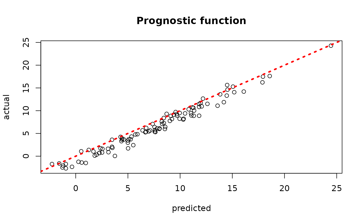
plot(rowMeans(bcf_model_warmstart$tau_hat_test), tau_test,
     xlab = "predicted", ylab = "actual", main = "Treatment effect")
abline(0,1,col="red",lty=3,lwd=3)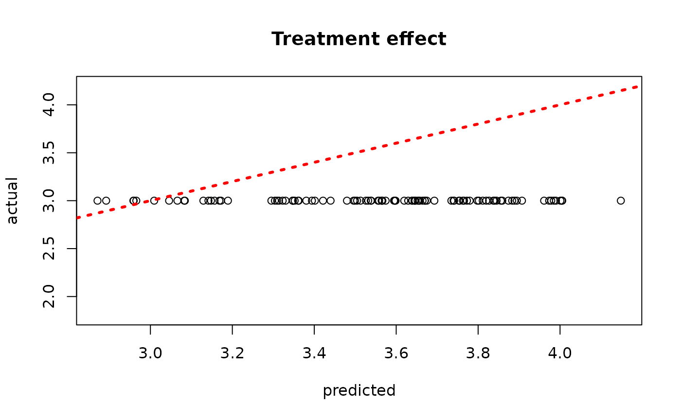
sigma_observed <- var(y-E_XZ)
plot_bounds <- c(min(c(bcf_model_warmstart$sigma2_samples, sigma_observed)),
                 max(c(bcf_model_warmstart$sigma2_samples, sigma_observed)))
plot(bcf_model_warmstart$sigma2_samples, ylim = plot_bounds,
     ylab = "sigma^2", xlab = "Sample", main = "Global variance parameter")
abline(h = sigma_observed, lty=3, lwd = 3, col = "blue")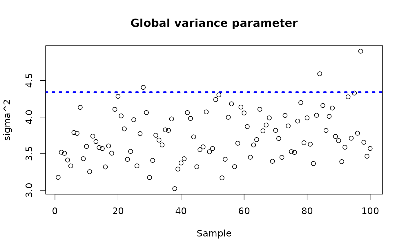
Examine test set interval coverage
BART MCMC without Warmstart
Next, we simulate from this ensemble model without any warm-start initialization.
num_gfr <- 0
num_burnin <- 100
num_mcmc <- 100
num_samples <- num_gfr + num_burnin + num_mcmc
bcf_params <- list(sample_sigma_leaf_mu = F, sample_sigma_leaf_tau = F,
                   keep_every = 5)
bcf_model_root <- bcf(
    X_train = X_train, Z_train = Z_train, y_train = y_train, pi_train = pi_train,
    X_test = X_test, Z_test = Z_test, pi_test = pi_test,
    num_gfr = num_gfr, num_burnin = num_burnin, num_mcmc = num_mcmc,
    params = bcf_params
)
Inspect the BART samples after burnin
plot(rowMeans(bcf_model_root$mu_hat_test), mu_test,
     xlab = "predicted", ylab = "actual", main = "Prognostic function")
abline(0,1,col="red",lty=3,lwd=3)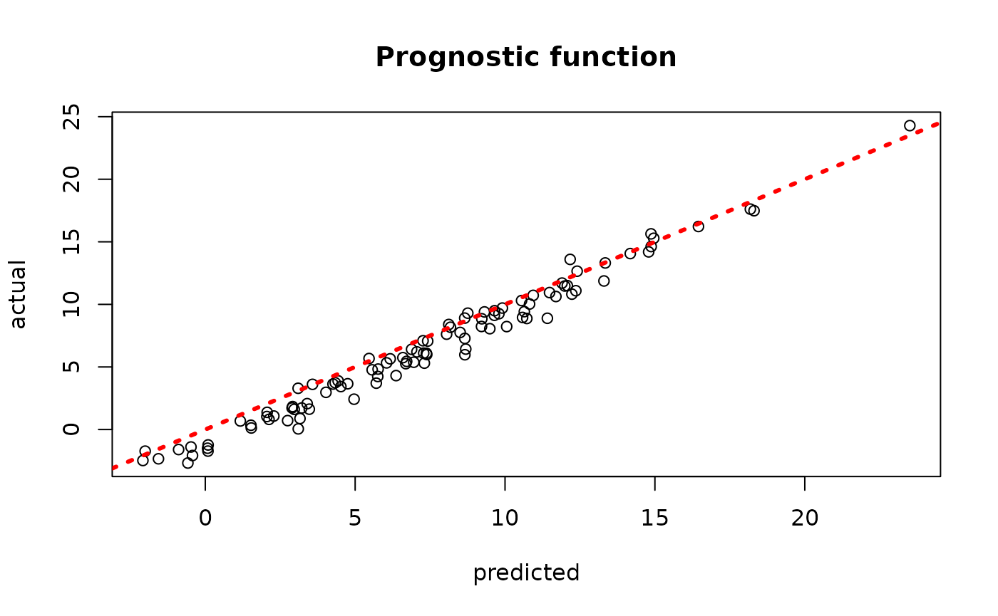
plot(rowMeans(bcf_model_root$tau_hat_test), tau_test,
     xlab = "predicted", ylab = "actual", main = "Treatment effect")
abline(0,1,col="red",lty=3,lwd=3)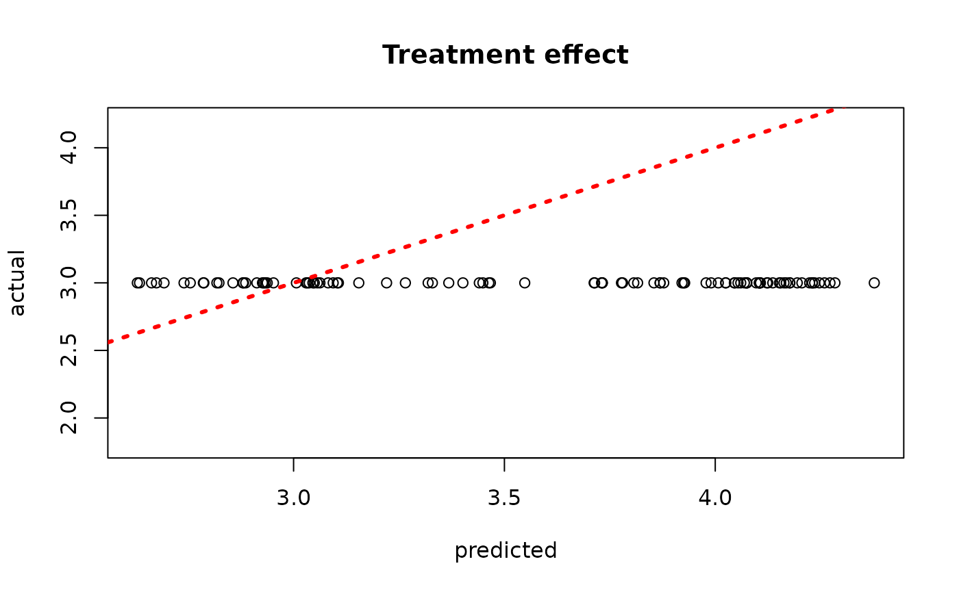
sigma_observed <- var(y-E_XZ)
plot_bounds <- c(min(c(bcf_model_root$sigma2_samples, sigma_observed)),
                 max(c(bcf_model_root$sigma2_samples, sigma_observed)))
plot(bcf_model_root$sigma2_samples, ylim = plot_bounds,
     ylab = "sigma^2", xlab = "Sample", main = "Global variance parameter")
abline(h = sigma_observed, lty=3, lwd = 3, col = "blue")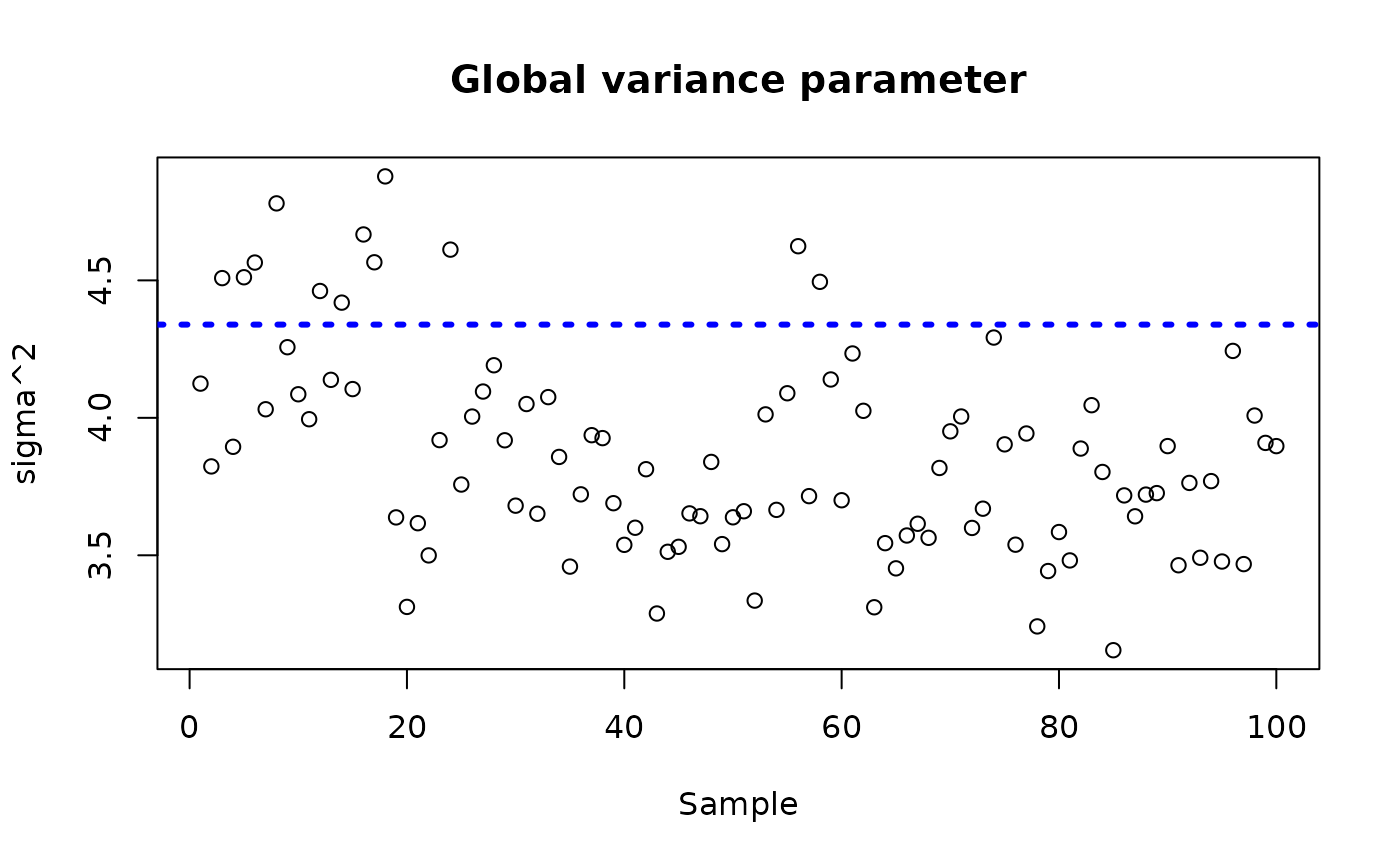
Examine test set interval coverage
Demo 4: Nonlinear Outcome Model, Heterogeneous Treatment Effect
We consider the following data generating process:
Simulation
We draw from the DGP defined above
n <- 1000
x1 <- rnorm(n)
x2 <- rnorm(n)
x3 <- rnorm(n)
x4 <- rnorm(n,x2,1)
X <- cbind(x1,x2,x3,x4)
p <- ncol(X)
mu <- function(x) {-1*(x[,1]>(x[,2])) + 1*(x[,1]<(x[,2])) - 0.1}
tau <- function(x) {1/(1 + exp(-x[,3])) + x[,2]/10}
mu_x <- mu(X)
tau_x <- tau(X)
pi_x <- pnorm(mu_x)
Z <- rbinom(n,1,pi_x)
E_XZ <- mu_x + Z*tau_x
sigma <- diff(range(mu_x + tau_x*pi))/8
y <- E_XZ + sigma*rnorm(n)
X <- as.data.frame(X)

# Split data into test and train sets
test_set_pct <- 0.2
n_test <- round(test_set_pct*n)
n_train <- n - n_test
test_inds <- sort(sample(1:n, n_test, replace = FALSE))
train_inds <- (1:n)[!((1:n) %in% test_inds)]
X_test <- X[test_inds,]
X_train <- X[train_inds,]
pi_test <- pi_x[test_inds]
pi_train <- pi_x[train_inds]
Z_test <- Z[test_inds]
Z_train <- Z[train_inds]
y_test <- y[test_inds]
y_train <- y[train_inds]
mu_test <- mu_x[test_inds]
mu_train <- mu_x[train_inds]
tau_test <- tau_x[test_inds]
tau_train <- tau_x[train_inds]
Sampling and Analysis
Warmstart
We first simulate from an ensemble model of
using “warm-start” initialization samples (Krantsevich, He, and Hahn (2023)). This is the
default in stochtree.
num_gfr <- 10
num_burnin <- 0
num_mcmc <- 100
num_samples <- num_gfr + num_burnin + num_mcmc
bcf_params <- list(sample_sigma_leaf_mu = F, sample_sigma_leaf_tau = F,
                   keep_every = 5)
bcf_model_warmstart <- bcf(
    X_train = X_train, Z_train = Z_train, y_train = y_train, pi_train = pi_train,
    X_test = X_test, Z_test = Z_test, pi_test = pi_test,
    num_gfr = num_gfr, num_burnin = num_burnin, num_mcmc = num_mcmc,
    params = bcf_params
)
#> Warning in t(tau_hat_train_raw) * (b_1_samples - b_0_samples): longer object
#> length is not a multiple of shorter object length
#> Warning in t(tau_hat_test_raw) * (b_1_samples - b_0_samples): longer object
#> length is not a multiple of shorter object length
Inspect the BART samples that were initialized with an XBART warm-start
plot(rowMeans(bcf_model_warmstart$mu_hat_test), mu_test,
     xlab = "predicted", ylab = "actual", main = "Prognostic function")
abline(0,1,col="red",lty=3,lwd=3)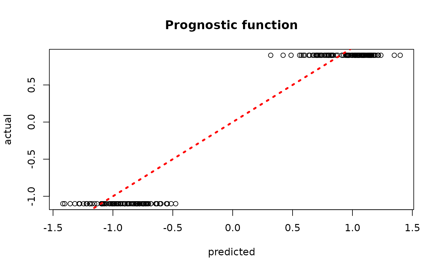
plot(rowMeans(bcf_model_warmstart$tau_hat_test), tau_test,
     xlab = "predicted", ylab = "actual", main = "Treatment effect")
abline(0,1,col="red",lty=3,lwd=3)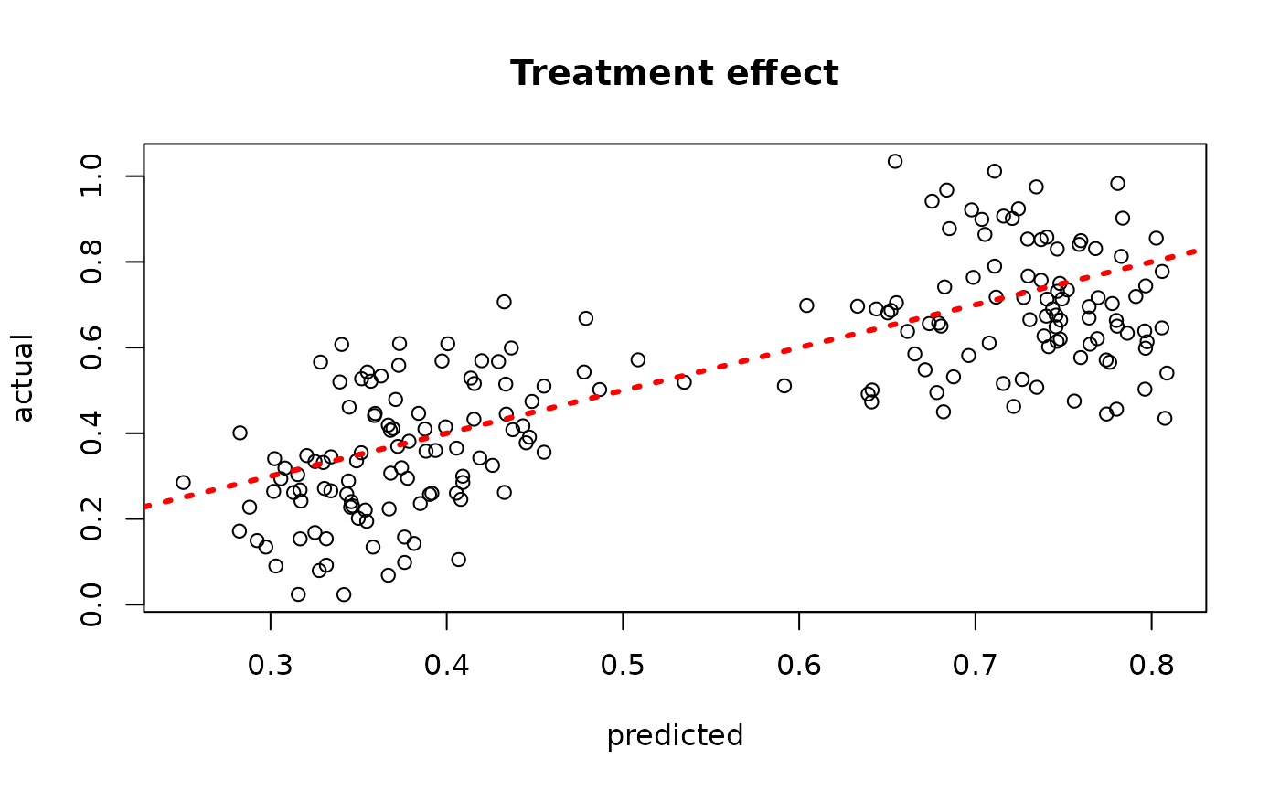
sigma_observed <- var(y-E_XZ)
plot_bounds <- c(min(c(bcf_model_warmstart$sigma2_samples, sigma_observed)),
                 max(c(bcf_model_warmstart$sigma2_samples, sigma_observed)))
plot(bcf_model_warmstart$sigma2_samples, ylim = plot_bounds,
     ylab = "sigma^2", xlab = "Sample", main = "Global variance parameter")
abline(h = sigma_observed, lty=3, lwd = 3, col = "blue")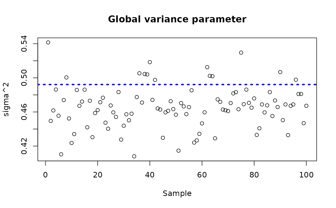
Examine test set interval coverage
BART MCMC without Warmstart
Next, we simulate from this ensemble model without any warm-start initialization.
num_gfr <- 0
num_burnin <- 100
num_mcmc <- 100
num_samples <- num_gfr + num_burnin + num_mcmc
bcf_params <- list(sample_sigma_leaf_mu = F, sample_sigma_leaf_tau = F,
                   keep_every = 5)
bcf_model_root <- bcf(
    X_train = X_train, Z_train = Z_train, y_train = y_train, pi_train = pi_train,
    X_test = X_test, Z_test = Z_test, pi_test = pi_test,
    num_gfr = num_gfr, num_burnin = num_burnin, num_mcmc = num_mcmc,
    params = bcf_params
)
Inspect the BART samples after burnin
plot(rowMeans(bcf_model_root$mu_hat_test), mu_test,
     xlab = "predicted", ylab = "actual", main = "Prognostic function")
abline(0,1,col="red",lty=3,lwd=3)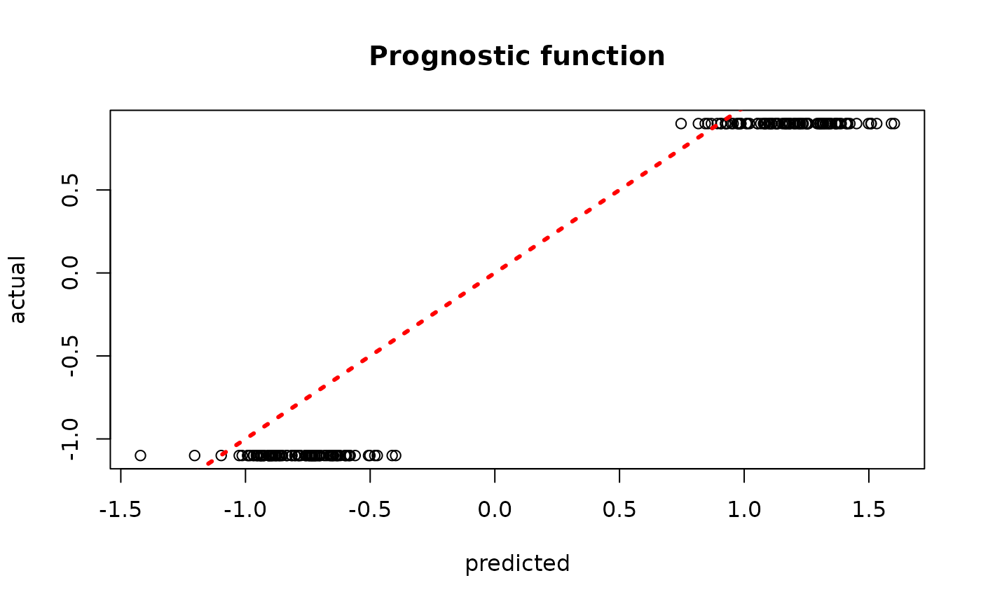
plot(rowMeans(bcf_model_root$tau_hat_test), tau_test,
     xlab = "predicted", ylab = "actual", main = "Treatment effect")
abline(0,1,col="red",lty=3,lwd=3)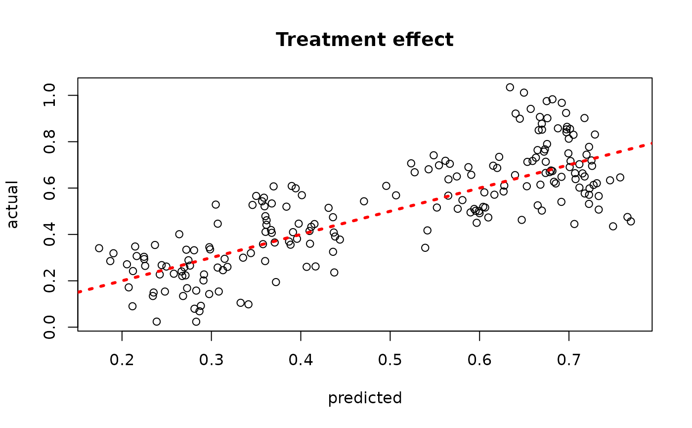
sigma_observed <- var(y-E_XZ)
plot_bounds <- c(min(c(bcf_model_root$sigma2_samples, sigma_observed)),
                 max(c(bcf_model_root$sigma2_samples, sigma_observed)))
plot(bcf_model_root$sigma2_samples, ylim = plot_bounds,
     ylab = "sigma^2", xlab = "Sample", main = "Global variance parameter")
abline(h = sigma_observed, lty=3, lwd = 3, col = "blue")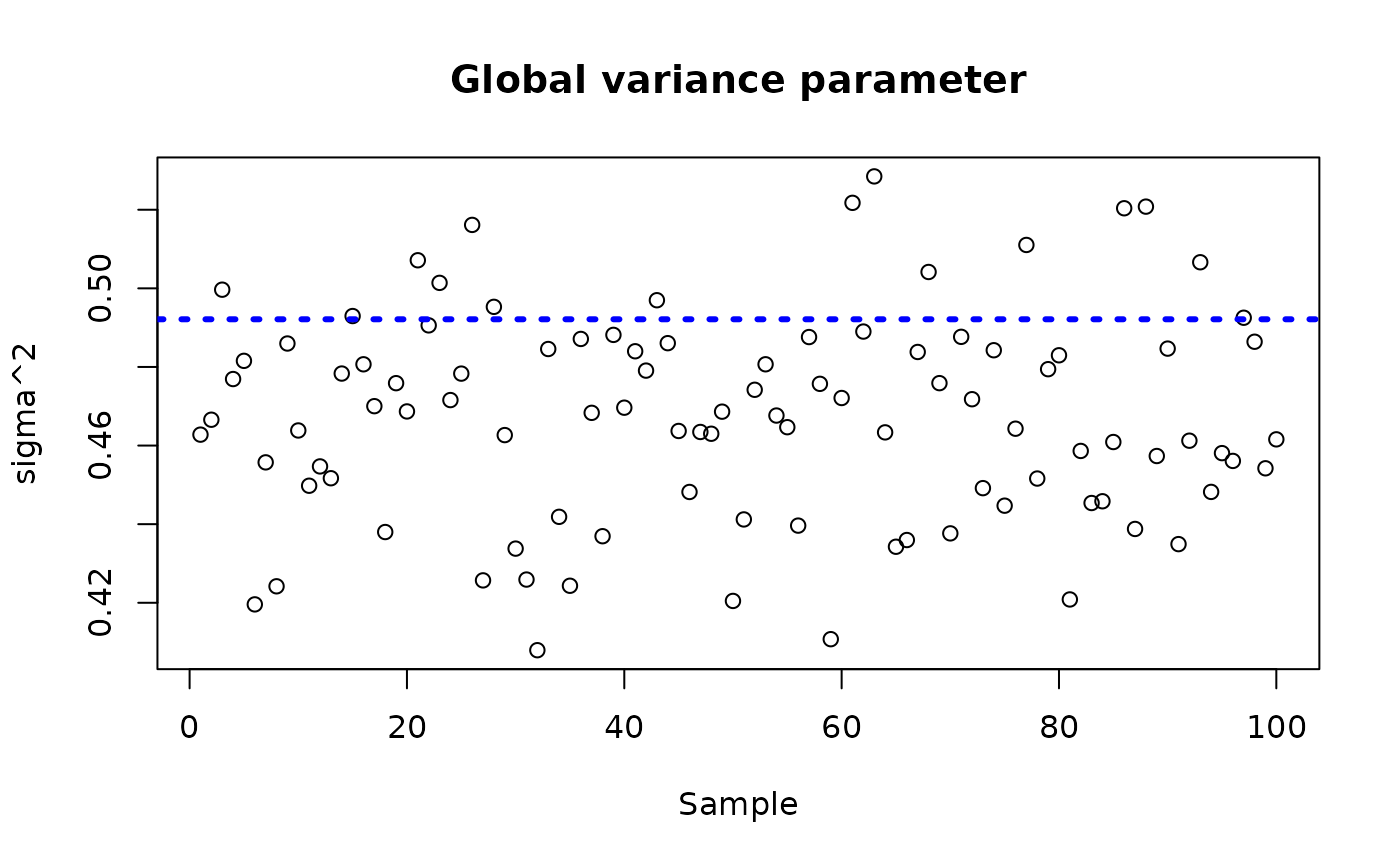
Examine test set interval coverage
Demo 5: Nonlinear Outcome Model, Heterogeneous Treatment Effect with Additive Random Effects
We augment the simulated example in Demo 1 with an additive random
effect structure and show that the bcf() function can
estimate and incorporate these effects into its forest sampling
procedure.
Simulation
We draw from the augmented “demo 1” DGP
n <- 500
snr <- 3
x1 <- rnorm(n)
x2 <- rnorm(n)
x3 <- rnorm(n)
x4 <- as.numeric(rbinom(n,1,0.5))
x5 <- as.numeric(sample(1:3,n,replace=TRUE))
X <- cbind(x1,x2,x3,x4,x5)
p <- ncol(X)
mu_x <- mu1(X)
tau_x <- tau2(X)
pi_x <- 0.8*pnorm((3*mu_x/sd(mu_x)) - 0.5*X[,1]) + 0.05 + runif(n)/10
Z <- rbinom(n,1,pi_x)
E_XZ <- mu_x + Z*tau_x
group_ids <- rep(c(1,2), n %/% 2)
rfx_coefs <- matrix(c(-1, -1, 1, 1), nrow=2, byrow=TRUE)
rfx_basis <- cbind(1, runif(n, -1, 1))
rfx_term <- rowSums(rfx_coefs[group_ids,] * rfx_basis)
y <- E_XZ + rfx_term + rnorm(n, 0, 1)*(sd(E_XZ)/snr)
X <- as.data.frame(X)
X$x4 <- factor(X$x4, ordered = TRUE)
X$x5 <- factor(X$x5, ordered = TRUE)

# Split data into test and train sets
test_set_pct <- 0.2
n_test <- round(test_set_pct*n)
n_train <- n - n_test
test_inds <- sort(sample(1:n, n_test, replace = FALSE))
train_inds <- (1:n)[!((1:n) %in% test_inds)]
X_test <- X[test_inds,]
X_train <- X[train_inds,]
pi_test <- pi_x[test_inds]
pi_train <- pi_x[train_inds]
Z_test <- Z[test_inds]
Z_train <- Z[train_inds]
y_test <- y[test_inds]
y_train <- y[train_inds]
mu_test <- mu_x[test_inds]
mu_train <- mu_x[train_inds]
tau_test <- tau_x[test_inds]
tau_train <- tau_x[train_inds]
group_ids_test <- group_ids[test_inds]
group_ids_train <- group_ids[train_inds]
rfx_basis_test <- rfx_basis[test_inds,]
rfx_basis_train <- rfx_basis[train_inds,]
rfx_term_test <- rfx_term[test_inds]
rfx_term_train <- rfx_term[train_inds]
Sampling and Analysis
Warmstart
Here we simulate only from the “warm-start” model (running root-MCMC
BART with random effects is simply a matter of modifying the below code
snippet by setting num_gfr <- 0 and
num_mcmc > 0).
num_gfr <- 100
num_burnin <- 0
num_mcmc <- 500
num_samples <- num_gfr + num_burnin + num_mcmc
bcf_params <- list(sample_sigma_leaf_mu = F, sample_sigma_leaf_tau = F,
                   keep_every = 5)
bcf_model_warmstart <- bcf(
    X_train = X_train, Z_train = Z_train, y_train = y_train, pi_train = pi_train,
    group_ids_train = group_ids_train, rfx_basis_train = rfx_basis_train,
    X_test = X_test, Z_test = Z_test, pi_test = pi_test, group_ids_test = group_ids_test,
    rfx_basis_test = rfx_basis_test, num_gfr = num_gfr, num_burnin = num_burnin, num_mcmc = num_mcmc,
    params = bcf_params
)
#> Warning in t(tau_hat_train_raw) * (b_1_samples - b_0_samples): longer object
#> length is not a multiple of shorter object length
#> Warning in t(tau_hat_test_raw) * (b_1_samples - b_0_samples): longer object
#> length is not a multiple of shorter object length
Inspect the BART samples that were initialized with an XBART warm-start
plot(rowMeans(bcf_model_warmstart$mu_hat_test), mu_test,
     xlab = "predicted", ylab = "actual", main = "Prognostic function")
abline(0,1,col="red",lty=3,lwd=3)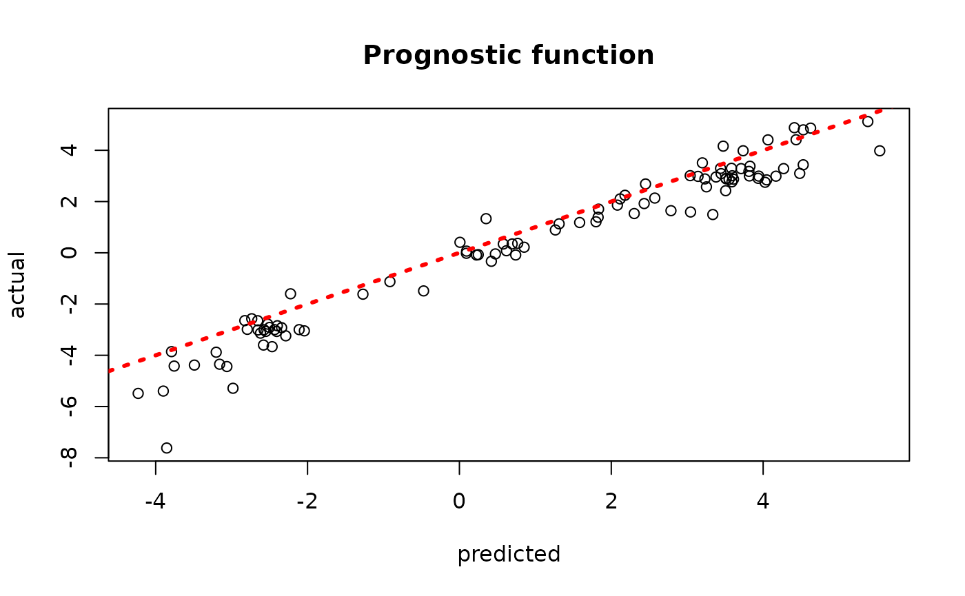
plot(rowMeans(bcf_model_warmstart$tau_hat_test), tau_test,
     xlab = "predicted", ylab = "actual", main = "Treatment effect")
abline(0,1,col="red",lty=3,lwd=3)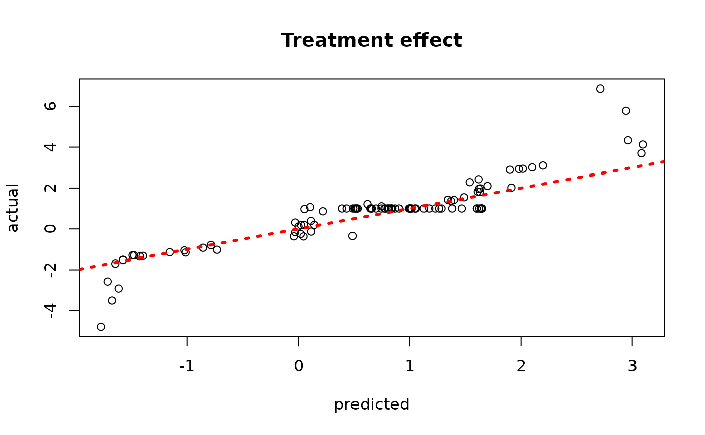
plot(rowMeans(bcf_model_warmstart$y_hat_test), y_test,
     xlab = "predicted", ylab = "actual", main = "Outcome")
abline(0,1,col="red",lty=3,lwd=3)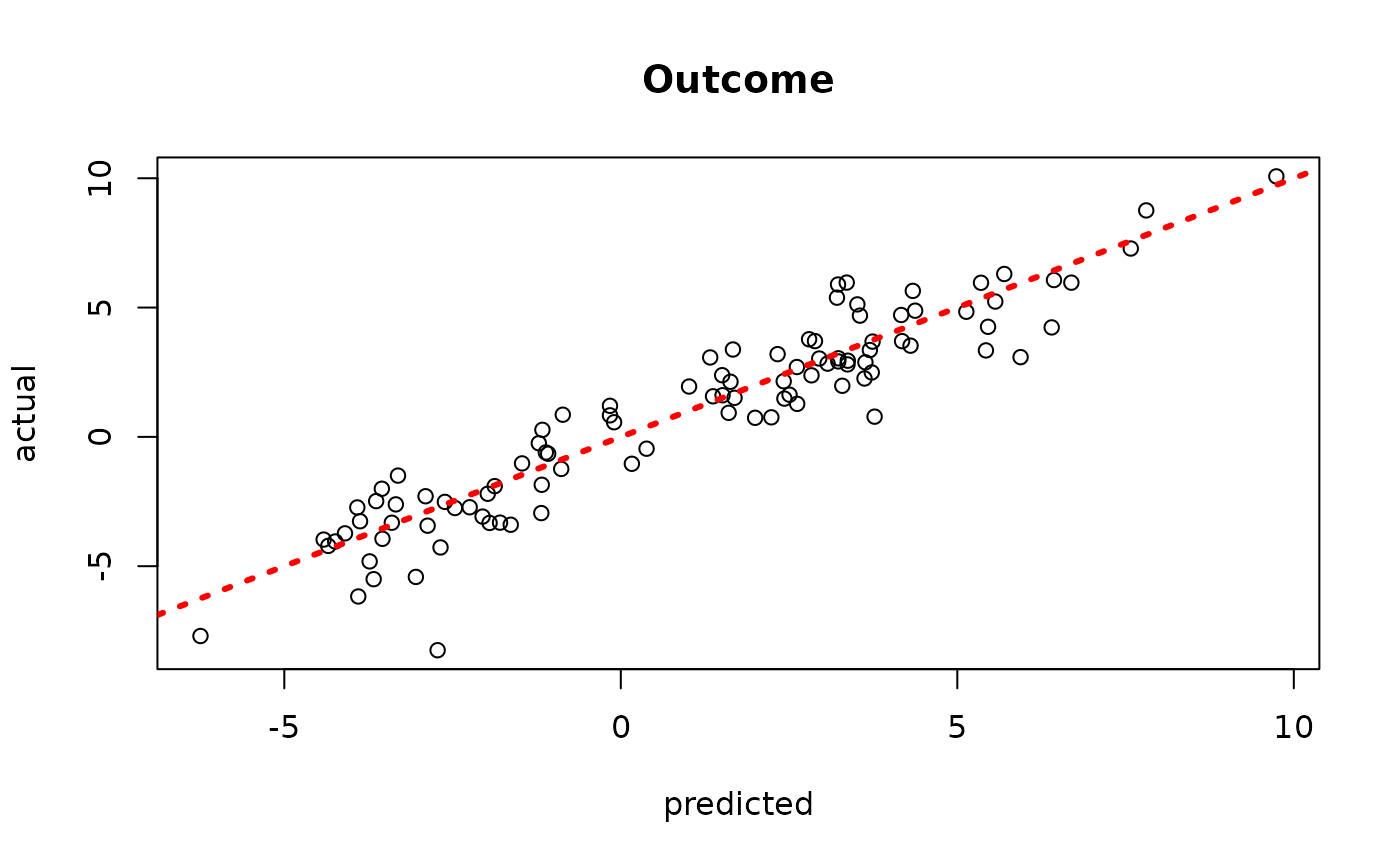
plot(rowMeans(bcf_model_warmstart$rfx_preds_test), rfx_term_test,
     xlab = "predicted", ylab = "actual", main = "Random effects terms")
abline(0,1,col="red",lty=3,lwd=3)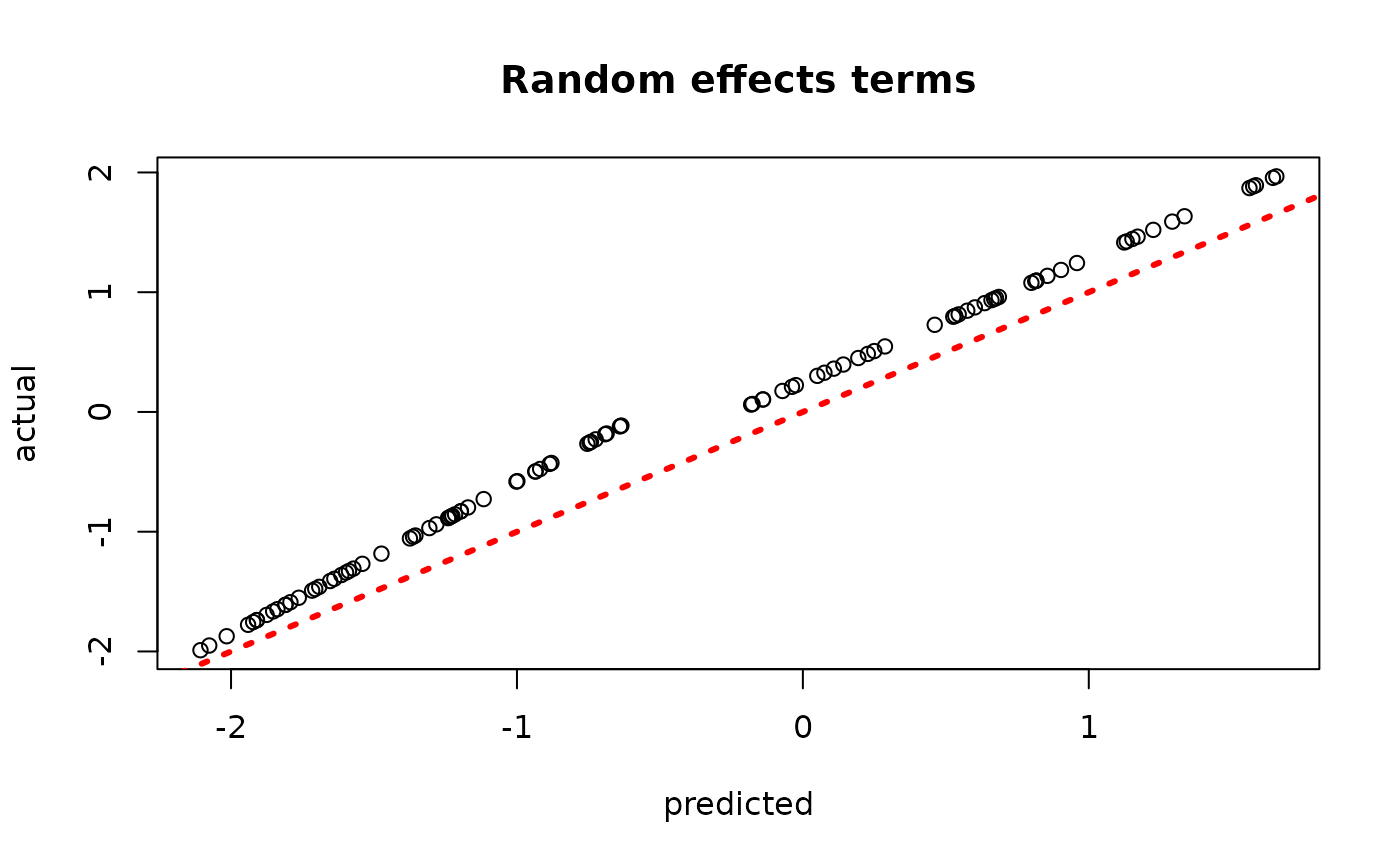
sigma_observed <- var(y-E_XZ-rfx_term)
plot_bounds <- c(min(c(bcf_model_warmstart$sigma2_samples, sigma_observed)),
                 max(c(bcf_model_warmstart$sigma2_samples, sigma_observed)))
plot(bcf_model_warmstart$sigma2_samples, ylim = plot_bounds,
     ylab = "sigma^2", xlab = "Sample", main = "Global variance parameter")
abline(h = sigma_observed, lty=3, lwd = 3, col = "blue")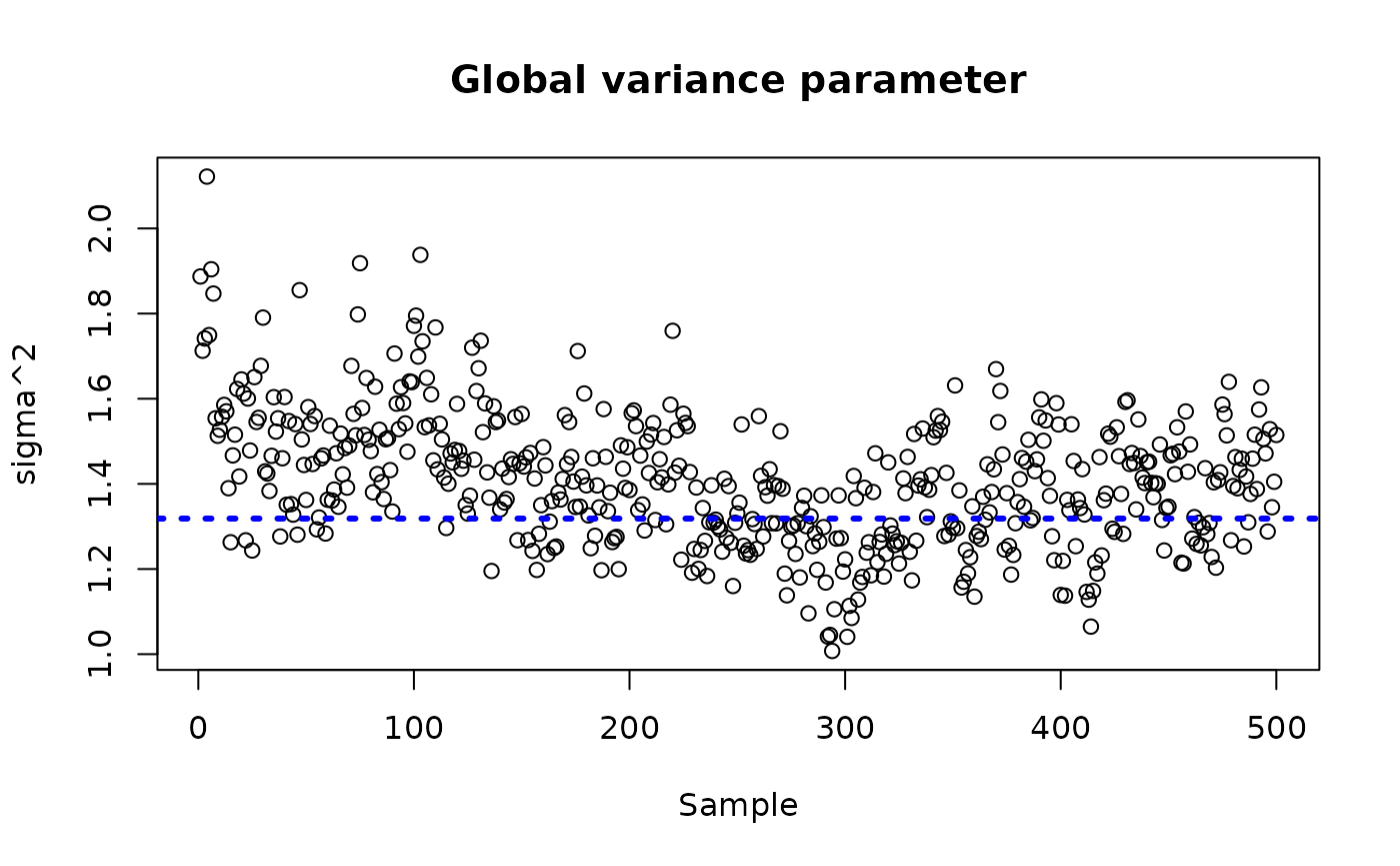
Examine test set interval coverage
test_lb <- apply(bcf_model_warmstart$tau_hat_test, 1, quantile, 0.025)
test_ub <- apply(bcf_model_warmstart$tau_hat_test, 1, quantile, 0.975)
cover <- (
    (test_lb <= tau_x[test_inds]) &
    (test_ub >= tau_x[test_inds])
)
mean(cover)
#> [1] 0.96
It is clear that causal inference is much more difficult in the presence of both strong covariate-dependent prognostic effects and strong group-level random effects. In this sense, proper prior calibration for all three of the , and random effects models is crucial.
Demo 6: Nonlinear Outcome Model, Heterogeneous Treatment Effect using Different Features in the Prognostic and Treatment Forests
Here, we consider the case in which we might prefer to use only a subset of covariates in the treatment effect forest. Why might we want to do that? Well, in many cases it is plausible that some covariates (for example age, income, etc…) influence the outcome of interest in a causal problem, but do not moderate the treatment effect. In this case, we’d need to include these variables in the prognostic forest for deconfounding but we don’t necessarily need to include them in the treatment effect forest.
Simulation
We draw from a modified “demo 1” DGP
mu <- function(x) {1+g(x)+x[,1]*x[,3]-x[,2]+3*x[,3]}
tau <- function(x) {1 - 2*x[,1] + 2*x[,2] + 1*x[,1]*x[,2]}
n <- 500
snr <- 4
x1 <- rnorm(n)
x2 <- rnorm(n)
x3 <- rnorm(n)
x4 <- as.numeric(rbinom(n,1,0.5))
x5 <- as.numeric(sample(1:3,n,replace=TRUE))
x6 <- rnorm(n)
x7 <- rnorm(n)
x8 <- rnorm(n)
x9 <- rnorm(n)
x10 <- rnorm(n)
X <- cbind(x1,x2,x3,x4,x5,x6,x7,x8,x9,x10)
p <- ncol(X)
mu_x <- mu(X)
tau_x <- tau(X)
pi_x <- 0.8*pnorm((3*mu_x/sd(mu_x)) - 0.5*X[,1]) + 0.05 + runif(n)/10
Z <- rbinom(n,1,pi_x)
E_XZ <- mu_x + Z*tau_x
y <- E_XZ + rnorm(n, 0, 1)*(sd(E_XZ)/snr)
X <- as.data.frame(X)
X$x4 <- factor(X$x4, ordered = TRUE)
X$x5 <- factor(X$x5, ordered = TRUE)

# Split data into test and train sets
test_set_pct <- 0.5
n_test <- round(test_set_pct*n)
n_train <- n - n_test
test_inds <- sort(sample(1:n, n_test, replace = FALSE))
train_inds <- (1:n)[!((1:n) %in% test_inds)]
X_test <- X[test_inds,]
X_train <- X[train_inds,]
pi_test <- pi_x[test_inds]
pi_train <- pi_x[train_inds]
Z_test <- Z[test_inds]
Z_train <- Z[train_inds]
y_test <- y[test_inds]
y_train <- y[train_inds]
mu_test <- mu_x[test_inds]
mu_train <- mu_x[train_inds]
tau_test <- tau_x[test_inds]
tau_train <- tau_x[train_inds]
Sampling and Analysis
MCMC, full covariate set in
Here we simulate from the model with the original MCMC sampler, using all of the covariates in both the prognostic () and treatment effect () forests.
num_gfr <- 0
num_burnin <- 1000
num_mcmc <- 1000
num_samples <- num_gfr + num_burnin + num_mcmc
bcf_params <- list(sample_sigma_leaf_mu = F, sample_sigma_leaf_tau = F,
                   keep_every = 5)
bcf_model_mcmc <- bcf(
    X_train = X_train, Z_train = Z_train, y_train = y_train, pi_train = pi_train,
    X_test = X_test, Z_test = Z_test, pi_test = pi_test,
    num_gfr = num_gfr, num_burnin = num_burnin, num_mcmc = num_mcmc,
    params = bcf_params
)
Inspect the burned-in samples
plot(rowMeans(bcf_model_mcmc$mu_hat_test), mu_test,
     xlab = "predicted", ylab = "actual", main = "Prognostic function")
abline(0,1,col="red",lty=3,lwd=3)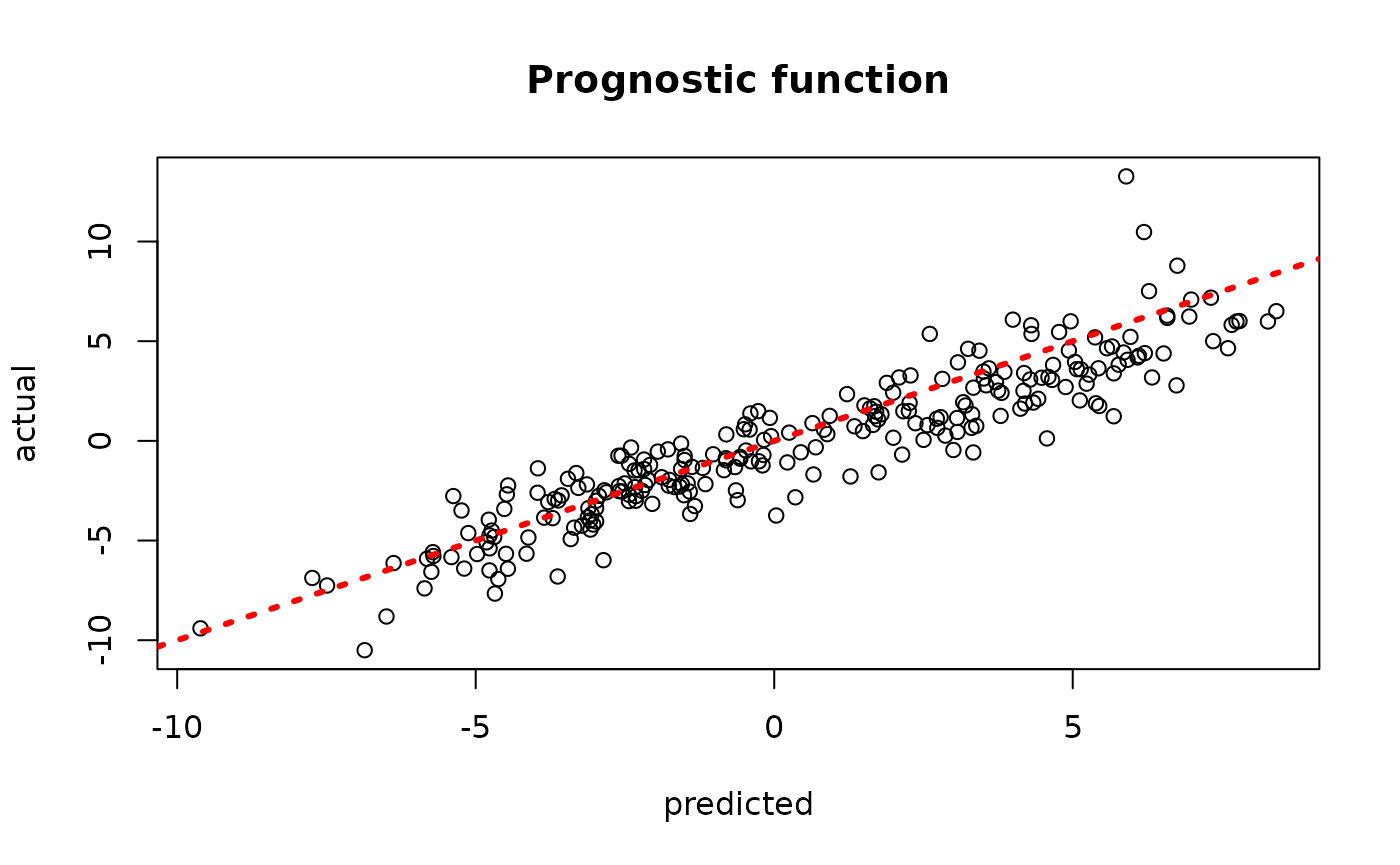
plot(rowMeans(bcf_model_mcmc$tau_hat_test), tau_test,
     xlab = "predicted", ylab = "actual", main = "Treatment effect")
abline(0,1,col="red",lty=3,lwd=3)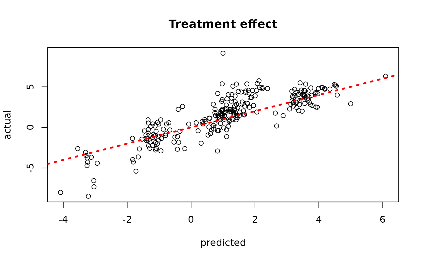
plot(rowMeans(bcf_model_mcmc$y_hat_test), y_test,
     xlab = "predicted", ylab = "actual", main = "Outcome")
abline(0,1,col="red",lty=3,lwd=3)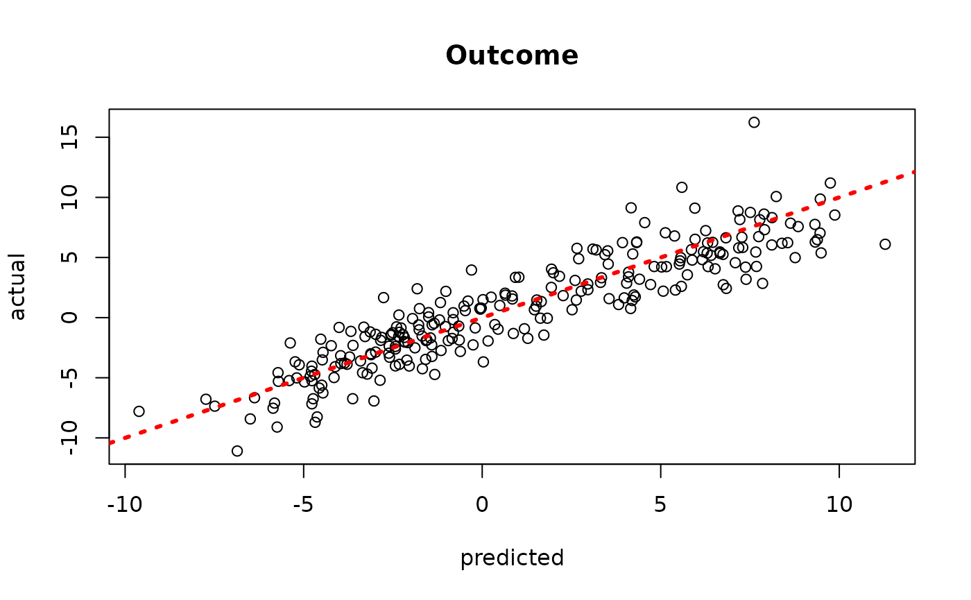
sigma_observed <- var(y-E_XZ)
plot_bounds <- c(min(c(bcf_model_mcmc$sigma2_samples, sigma_observed)),
                 max(c(bcf_model_mcmc$sigma2_samples, sigma_observed)))
plot(bcf_model_mcmc$sigma2_samples, ylim = plot_bounds,
     ylab = "sigma^2", xlab = "Sample", main = "Global variance parameter")
abline(h = sigma_observed, lty=3, lwd = 3, col = "blue")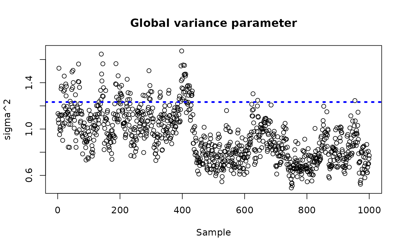
Examine test set interval coverage
test_lb <- apply(bcf_model_mcmc$tau_hat_test, 1, quantile, 0.025)
test_ub <- apply(bcf_model_mcmc$tau_hat_test, 1, quantile, 0.975)
cover <- (
    (test_lb <= tau_x[test_inds]) &
    (test_ub >= tau_x[test_inds])
)
mean(cover)
#> [1] 0.948
And test set RMSE
MCMC, covariate subset in
Here we simulate from the model with the original MCMC sampler, using only covariate in the treatment effect forest.
num_gfr <- 0
num_burnin <- 1000
num_mcmc <- 1000
num_samples <- num_gfr + num_burnin + num_mcmc
bcf_params <- list(sample_sigma_leaf_mu = F, sample_sigma_leaf_tau = F,
                   keep_vars_tau = c("x1","x2"), keep_every = 5)
bcf_model_mcmc <- bcf(
    X_train = X_train, Z_train = Z_train, y_train = y_train, pi_train = pi_train,
    X_test = X_test, Z_test = Z_test, pi_test = pi_test,
    num_gfr = num_gfr, num_burnin = num_burnin, num_mcmc = num_mcmc,
    params = bcf_params
)
Inspect the BART samples
plot(rowMeans(bcf_model_mcmc$mu_hat_test), mu_test,
     xlab = "predicted", ylab = "actual", main = "Prognostic function")
abline(0,1,col="red",lty=3,lwd=3)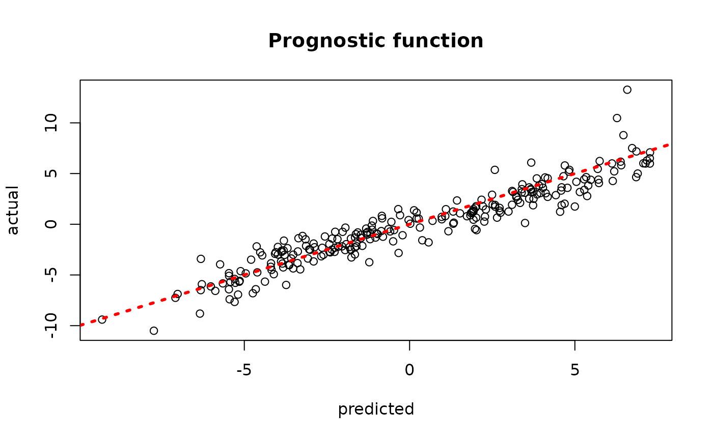
plot(rowMeans(bcf_model_mcmc$tau_hat_test), tau_test,
     xlab = "predicted", ylab = "actual", main = "Treatment effect")
abline(0,1,col="red",lty=3,lwd=3)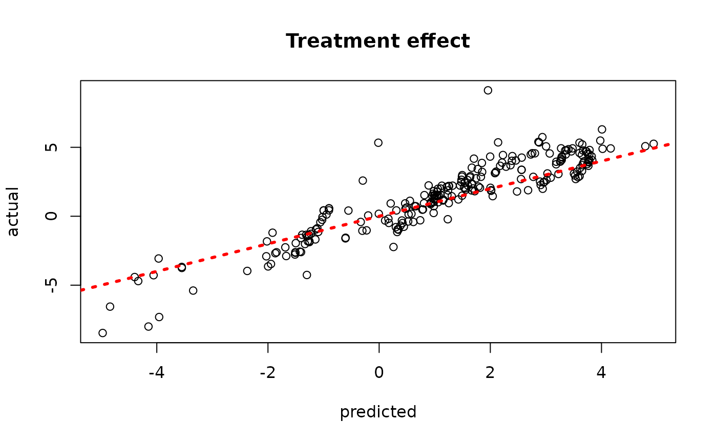
plot(rowMeans(bcf_model_mcmc$y_hat_test), y_test,
     xlab = "predicted", ylab = "actual", main = "Outcome")
abline(0,1,col="red",lty=3,lwd=3)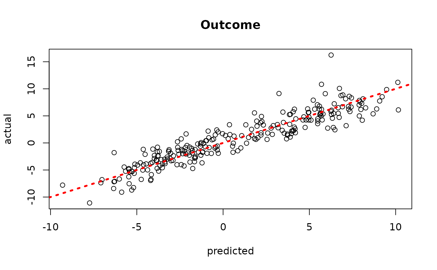
sigma_observed <- var(y-E_XZ)
plot_bounds <- c(min(c(bcf_model_mcmc$sigma2_samples, sigma_observed)),
                 max(c(bcf_model_mcmc$sigma2_samples, sigma_observed)))
plot(bcf_model_mcmc$sigma2_samples, ylim = plot_bounds,
     ylab = "sigma^2", xlab = "Sample", main = "Global variance parameter")
abline(h = sigma_observed, lty=3, lwd = 3, col = "blue")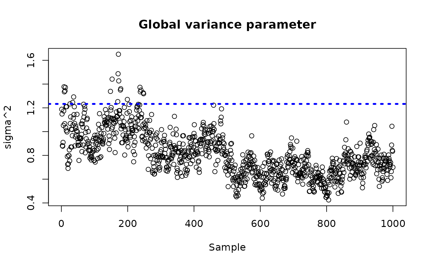
Examine test set interval coverage
test_lb <- apply(bcf_model_mcmc$tau_hat_test, 1, quantile, 0.025)
test_ub <- apply(bcf_model_mcmc$tau_hat_test, 1, quantile, 0.975)
cover <- (
    (test_lb <= tau_x[test_inds]) &
    (test_ub >= tau_x[test_inds])
)
mean(cover)
#> [1] 0.952
And test set RMSE
Warmstart, full covariate set in
Here we simulate from the model with the warm-start sampler, using all of the covariates in both the prognostic () and treatment effect () forests.
num_gfr <- 10
num_burnin <- 0
num_mcmc <- 1000
num_samples <- num_gfr + num_burnin + num_mcmc
bcf_params <- list(sample_sigma_leaf_mu = F, sample_sigma_leaf_tau = F,
                   keep_every = 5)
bcf_model_warmstart <- bcf(
    X_train = X_train, Z_train = Z_train, y_train = y_train, pi_train = pi_train,
    X_test = X_test, Z_test = Z_test, pi_test = pi_test,
    num_gfr = num_gfr, num_burnin = num_burnin, num_mcmc = num_mcmc,
    params = bcf_params
)
#> Warning in t(tau_hat_train_raw) * (b_1_samples - b_0_samples): longer object
#> length is not a multiple of shorter object length
#> Warning in t(tau_hat_test_raw) * (b_1_samples - b_0_samples): longer object
#> length is not a multiple of shorter object length
Inspect the BART samples that were initialized with an XBART warm-start
plot(rowMeans(bcf_model_warmstart$mu_hat_test), mu_test,
     xlab = "predicted", ylab = "actual", main = "Prognostic function")
abline(0,1,col="red",lty=3,lwd=3)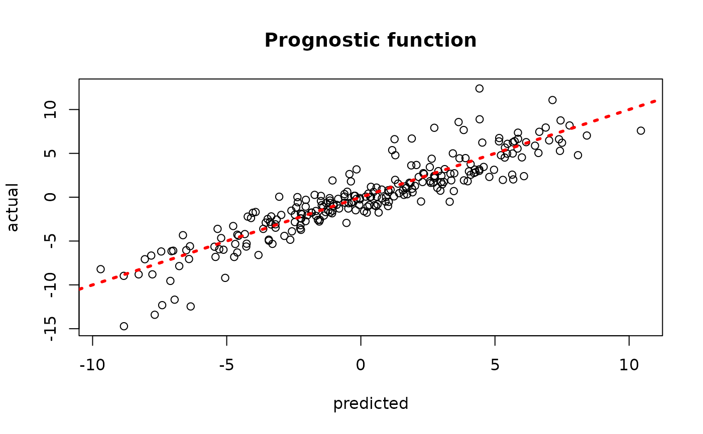
plot(rowMeans(bcf_model_warmstart$tau_hat_test), tau_test,
     xlab = "predicted", ylab = "actual", main = "Treatment effect")
abline(0,1,col="red",lty=3,lwd=3)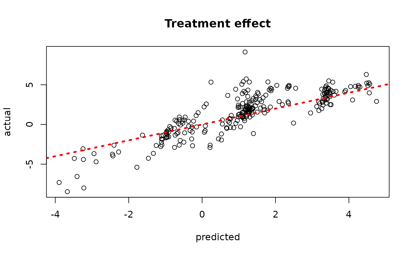
plot(rowMeans(bcf_model_warmstart$y_hat_test), y_test,
     xlab = "predicted", ylab = "actual", main = "Outcome")
abline(0,1,col="red",lty=3,lwd=3)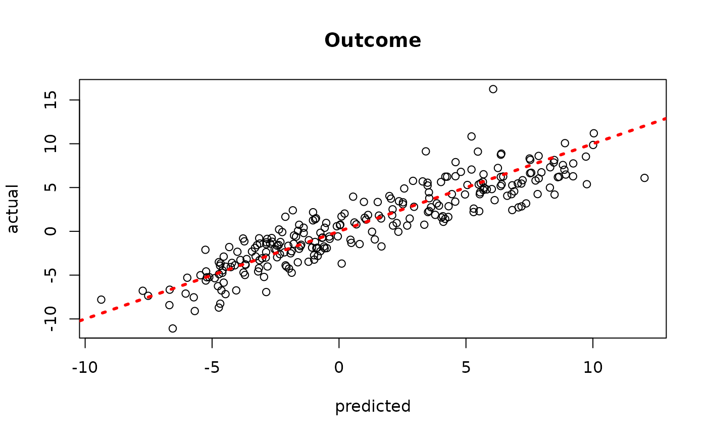
sigma_observed <- var(y-E_XZ)
plot_bounds <- c(min(c(bcf_model_warmstart$sigma2_samples, sigma_observed)),
                 max(c(bcf_model_warmstart$sigma2_samples, sigma_observed)))
plot(bcf_model_warmstart$sigma2_samples, ylim = plot_bounds,
     ylab = "sigma^2", xlab = "Sample", main = "Global variance parameter")
abline(h = sigma_observed, lty=3, lwd = 3, col = "blue")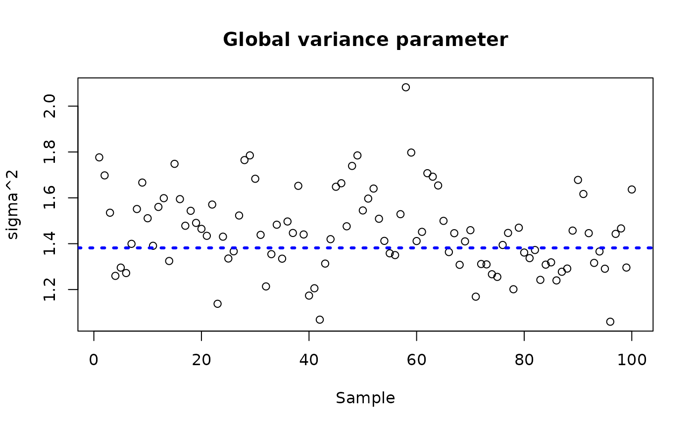
Examine test set interval coverage
test_lb <- apply(bcf_model_warmstart$tau_hat_test, 1, quantile, 0.025)
test_ub <- apply(bcf_model_warmstart$tau_hat_test, 1, quantile, 0.975)
cover <- (
    (test_lb <= tau_x[test_inds]) &
    (test_ub >= tau_x[test_inds])
)
mean(cover)
#> [1] 0.98
And test set RMSE
Warmstart, covariate subset in
Here we simulate from the model with the warm-start sampler, using only covariate in the treatment effect forest.
num_gfr <- 10
num_burnin <- 0
num_mcmc <- 1000
num_samples <- num_gfr + num_burnin + num_mcmc
bcf_params <- list(sample_sigma_leaf_mu = F, sample_sigma_leaf_tau = F,
                   keep_vars_tau = c("x1","x2"), keep_every = 5)
bcf_model_warmstart <- bcf(
    X_train = X_train, Z_train = Z_train, y_train = y_train, pi_train = pi_train,
    X_test = X_test, Z_test = Z_test, pi_test = pi_test,
    num_gfr = num_gfr, num_burnin = num_burnin, num_mcmc = num_mcmc,
    params = bcf_params
)
#> Warning in t(tau_hat_train_raw) * (b_1_samples - b_0_samples): longer object
#> length is not a multiple of shorter object length
#> Warning in t(tau_hat_test_raw) * (b_1_samples - b_0_samples): longer object
#> length is not a multiple of shorter object length
Inspect the BART samples that were initialized with an XBART warm-start
plot(rowMeans(bcf_model_warmstart$mu_hat_test), mu_test,
     xlab = "predicted", ylab = "actual", main = "Prognostic function")
abline(0,1,col="red",lty=3,lwd=3)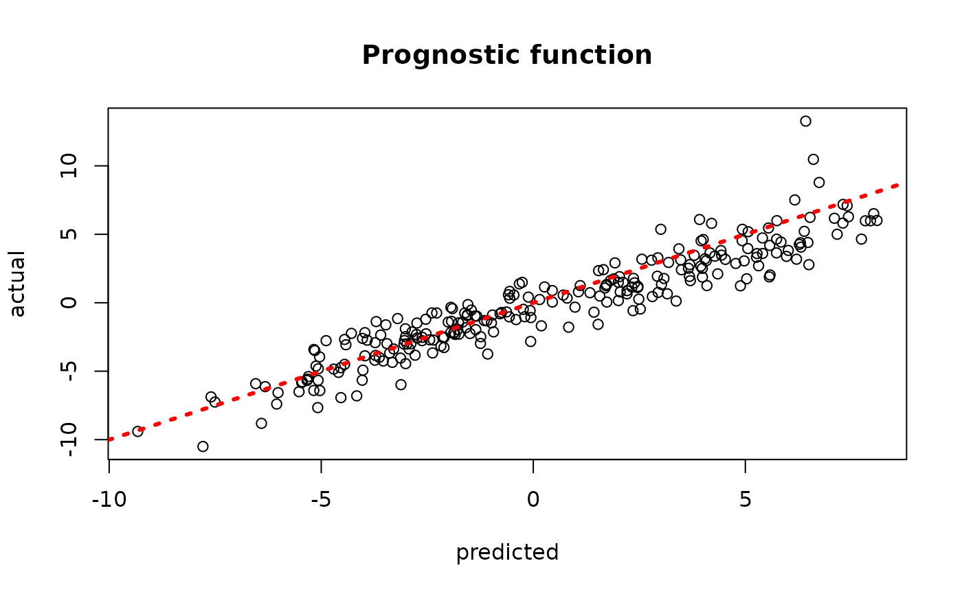
plot(rowMeans(bcf_model_warmstart$tau_hat_test), tau_test,
     xlab = "predicted", ylab = "actual", main = "Treatment effect")
abline(0,1,col="red",lty=3,lwd=3)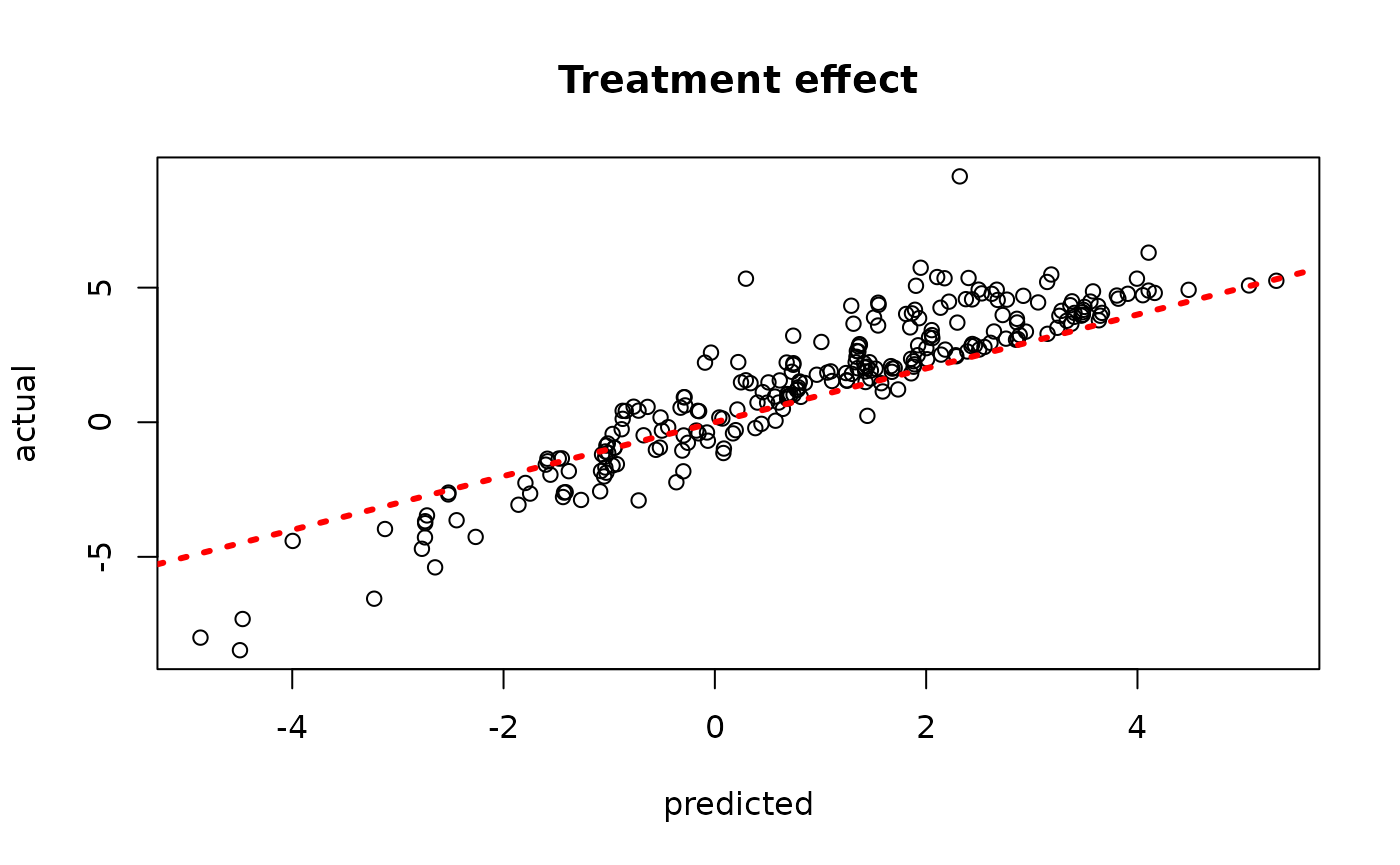
plot(rowMeans(bcf_model_warmstart$y_hat_test), y_test,
     xlab = "predicted", ylab = "actual", main = "Outcome")
abline(0,1,col="red",lty=3,lwd=3)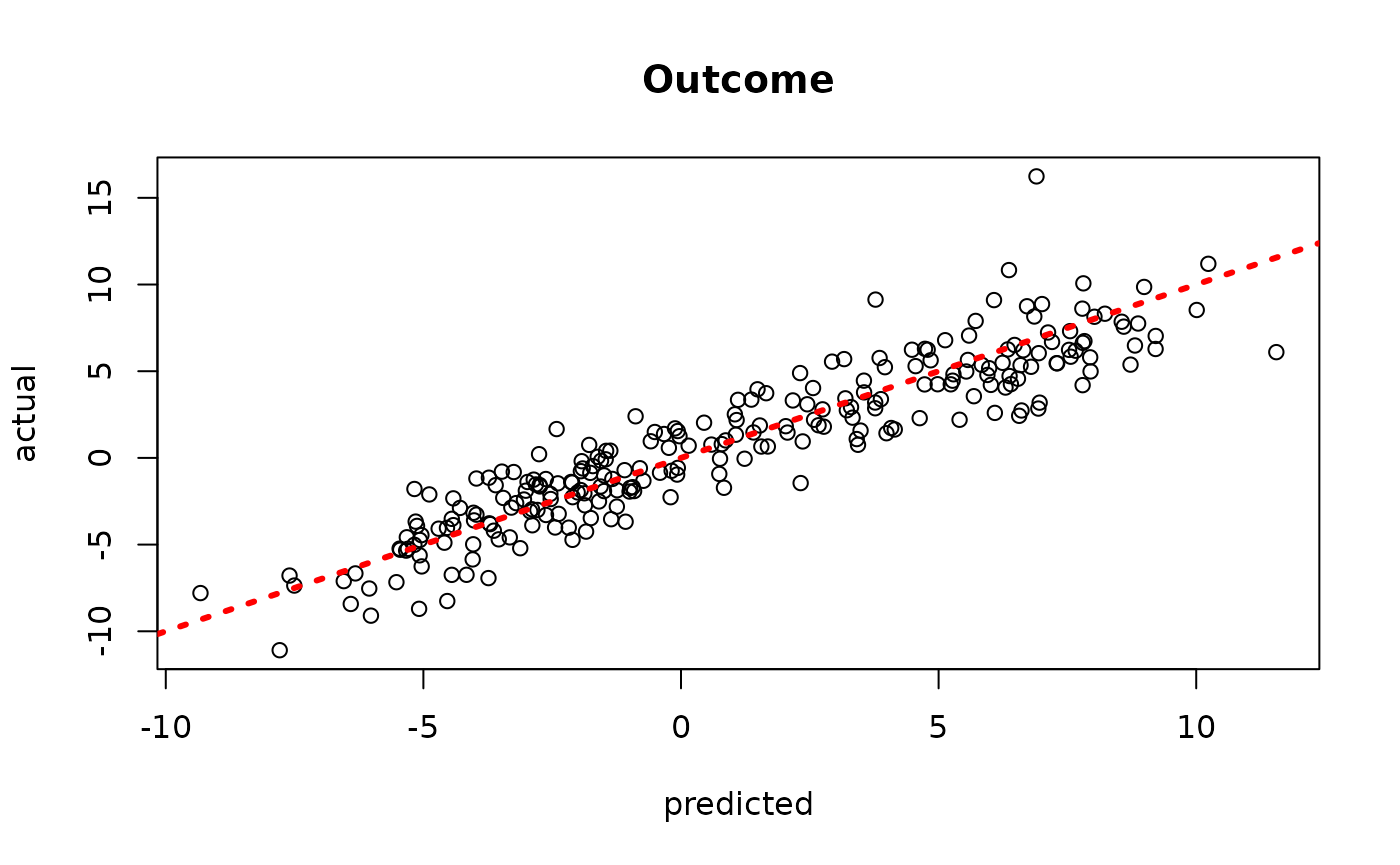
sigma_observed <- var(y-E_XZ)
plot_bounds <- c(min(c(bcf_model_warmstart$sigma2_samples, sigma_observed)),
                 max(c(bcf_model_warmstart$sigma2_samples, sigma_observed)))
plot(bcf_model_warmstart$sigma2_samples, ylim = plot_bounds,
     ylab = "sigma^2", xlab = "Sample", main = "Global variance parameter")
abline(h = sigma_observed, lty=3, lwd = 3, col = "blue")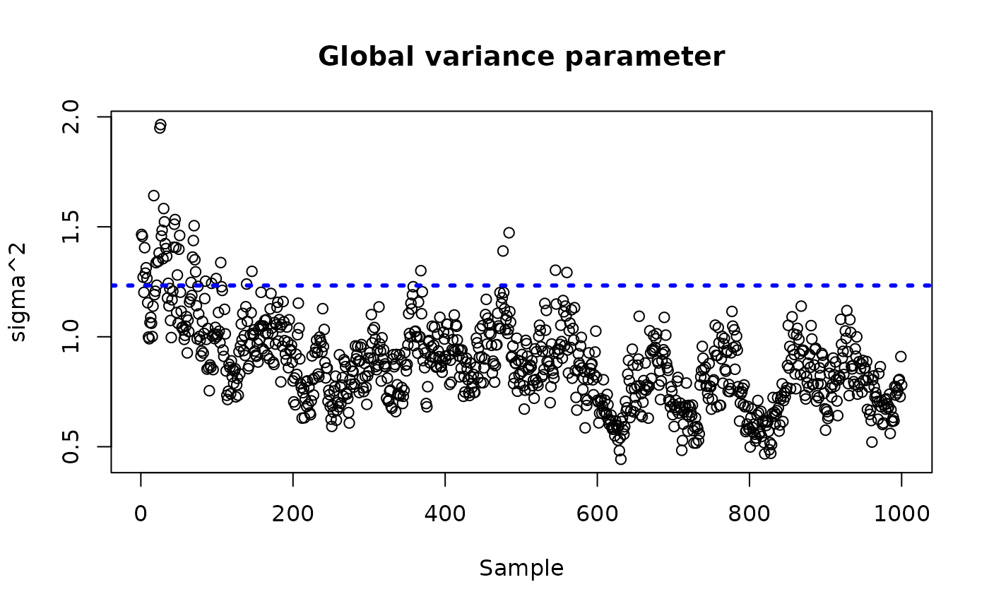
Examine test set interval coverage
test_lb <- apply(bcf_model_warmstart$tau_hat_test, 1, quantile, 0.025)
test_ub <- apply(bcf_model_warmstart$tau_hat_test, 1, quantile, 0.975)
cover <- (
    (test_lb <= tau_x[test_inds]) &
    (test_ub >= tau_x[test_inds])
)
mean(cover)
#> [1] 0.98
And test set RMSE
Continuous Treatment
Demo 1: Nonlinear Outcome Model, Heterogeneous Treatment Effect
We consider the following data generating process:
Simulation
We draw from the DGP defined above
n <- 500
snr <- 3
x1 <- rnorm(n)
x2 <- rnorm(n)
x3 <- rnorm(n)
x4 <- rnorm(n)
x5 <- rnorm(n)
X <- cbind(x1,x2,x3,x4,x5)
p <- ncol(X)
mu_x <- 1 + 2*x1 - 4*(x2 < 0) + 4*(x2 >= 0) + 3*(abs(x3) - sqrt(2/pi))
tau_x <- 1 + 2*x4
u <- runif(n)
pi_x <- ((mu_x-1)/4) + 4*(u-0.5)
Z <- pi_x + rnorm(n,0,1)
E_XZ <- mu_x + Z*tau_x
y <- E_XZ + rnorm(n, 0, 1)*(sd(E_XZ)/snr)
X <- as.data.frame(X)

# Split data into test and train sets
test_set_pct <- 0.2
n_test <- round(test_set_pct*n)
n_train <- n - n_test
test_inds <- sort(sample(1:n, n_test, replace = FALSE))
train_inds <- (1:n)[!((1:n) %in% test_inds)]
X_test <- X[test_inds,]
X_train <- X[train_inds,]
pi_test <- pi_x[test_inds]
pi_train <- pi_x[train_inds]
Z_test <- Z[test_inds]
Z_train <- Z[train_inds]
y_test <- y[test_inds]
y_train <- y[train_inds]
mu_test <- mu_x[test_inds]
mu_train <- mu_x[train_inds]
tau_test <- tau_x[test_inds]
tau_train <- tau_x[train_inds]
Sampling and Analysis
Warmstart
We first simulate from an ensemble model of
using “warm-start” initialization samples (Krantsevich, He, and Hahn (2023)). This is the
default in stochtree.
num_gfr <- 10
num_burnin <- 0
num_mcmc <- 1000
num_samples <- num_gfr + num_burnin + num_mcmc
bcf_params <- list(sample_sigma_leaf_mu = F, sample_sigma_leaf_tau = F,
                   keep_every = 5)
bcf_model_warmstart <- bcf(
    X_train = X_train, Z_train = Z_train, y_train = y_train, pi_train = pi_train,
    X_test = X_test, Z_test = Z_test, pi_test = pi_test,
    num_gfr = num_gfr, num_burnin = num_burnin, num_mcmc = num_mcmc,
    params = bcf_params
)
Inspect the BART samples that were initialized with an XBART warm-start
plot(rowMeans(bcf_model_warmstart$mu_hat_test), mu_test,
     xlab = "predicted", ylab = "actual", main = "Prognostic function")
abline(0,1,col="red",lty=3,lwd=3)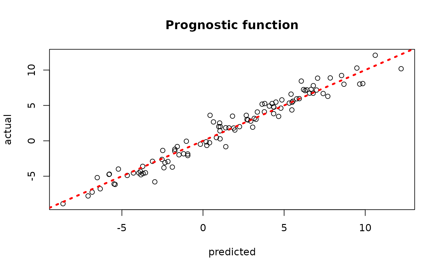
plot(rowMeans(bcf_model_warmstart$tau_hat_test), tau_test,
     xlab = "predicted", ylab = "actual", main = "Treatment effect")
abline(0,1,col="red",lty=3,lwd=3)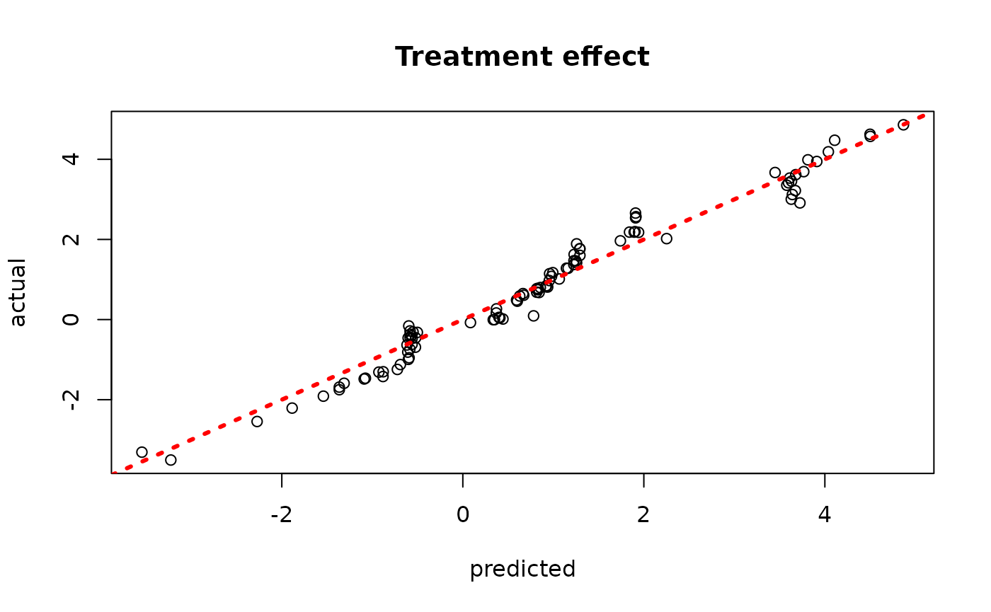
sigma_observed <- var(y-E_XZ)
plot_bounds <- c(min(c(bcf_model_warmstart$sigma2_samples, sigma_observed)),
                 max(c(bcf_model_warmstart$sigma2_samples, sigma_observed)))
plot(bcf_model_warmstart$sigma2_samples, ylim = plot_bounds,
     ylab = "sigma^2", xlab = "Sample", main = "Global variance parameter")
abline(h = sigma_observed, lty=3, lwd = 3, col = "blue")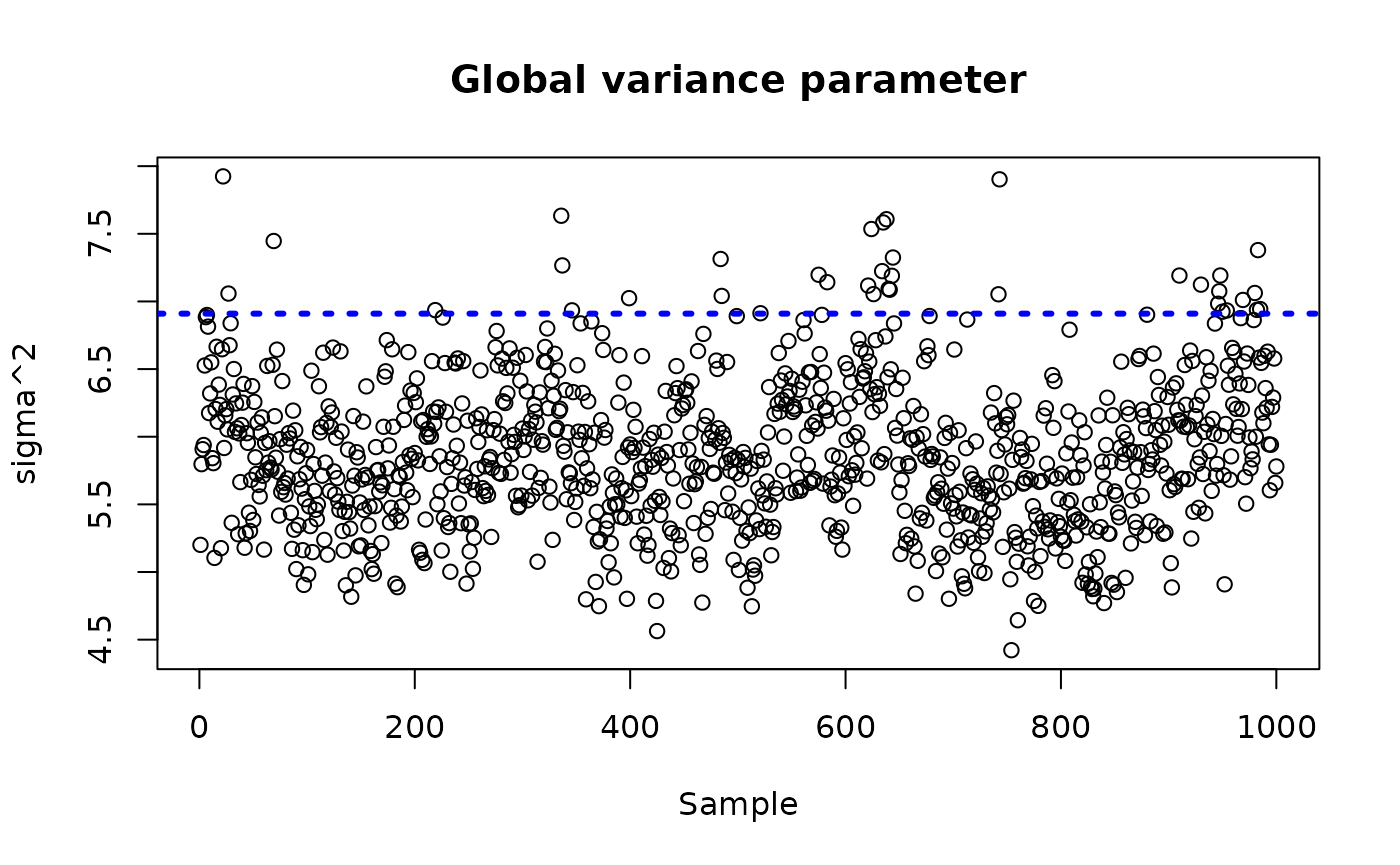
Examine test set interval coverage
BART MCMC without Warmstart
Next, we simulate from this ensemble model without any warm-start initialization.
num_gfr <- 0
num_burnin <- 1000
num_mcmc <- 1000
num_samples <- num_gfr + num_burnin + num_mcmc
bcf_params <- list(sample_sigma_leaf_mu = F, sample_sigma_leaf_tau = F,
                   keep_every = 5)
bcf_model_root <- bcf(
    X_train = X_train, Z_train = Z_train, y_train = y_train, pi_train = pi_train,
    X_test = X_test, Z_test = Z_test, pi_test = pi_test,
    num_gfr = num_gfr, num_burnin = num_burnin, num_mcmc = num_mcmc,
    params = bcf_params
)
Inspect the BART samples after burnin
plot(rowMeans(bcf_model_root$mu_hat_test), mu_test,
     xlab = "predicted", ylab = "actual", main = "Prognostic function")
abline(0,1,col="red",lty=3,lwd=3)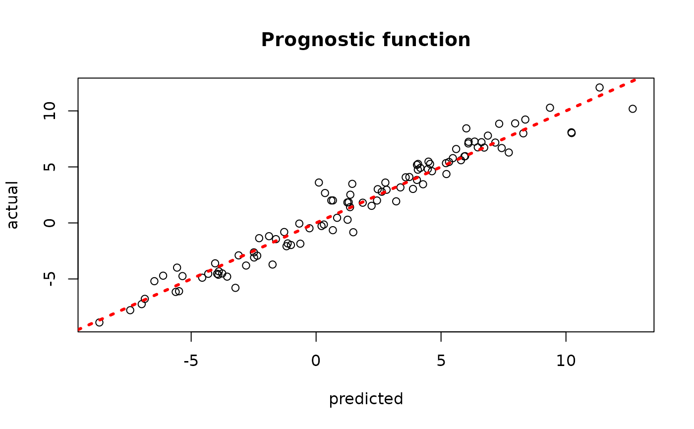
plot(rowMeans(bcf_model_root$tau_hat_test), tau_test,
     xlab = "predicted", ylab = "actual", main = "Treatment effect")
abline(0,1,col="red",lty=3,lwd=3)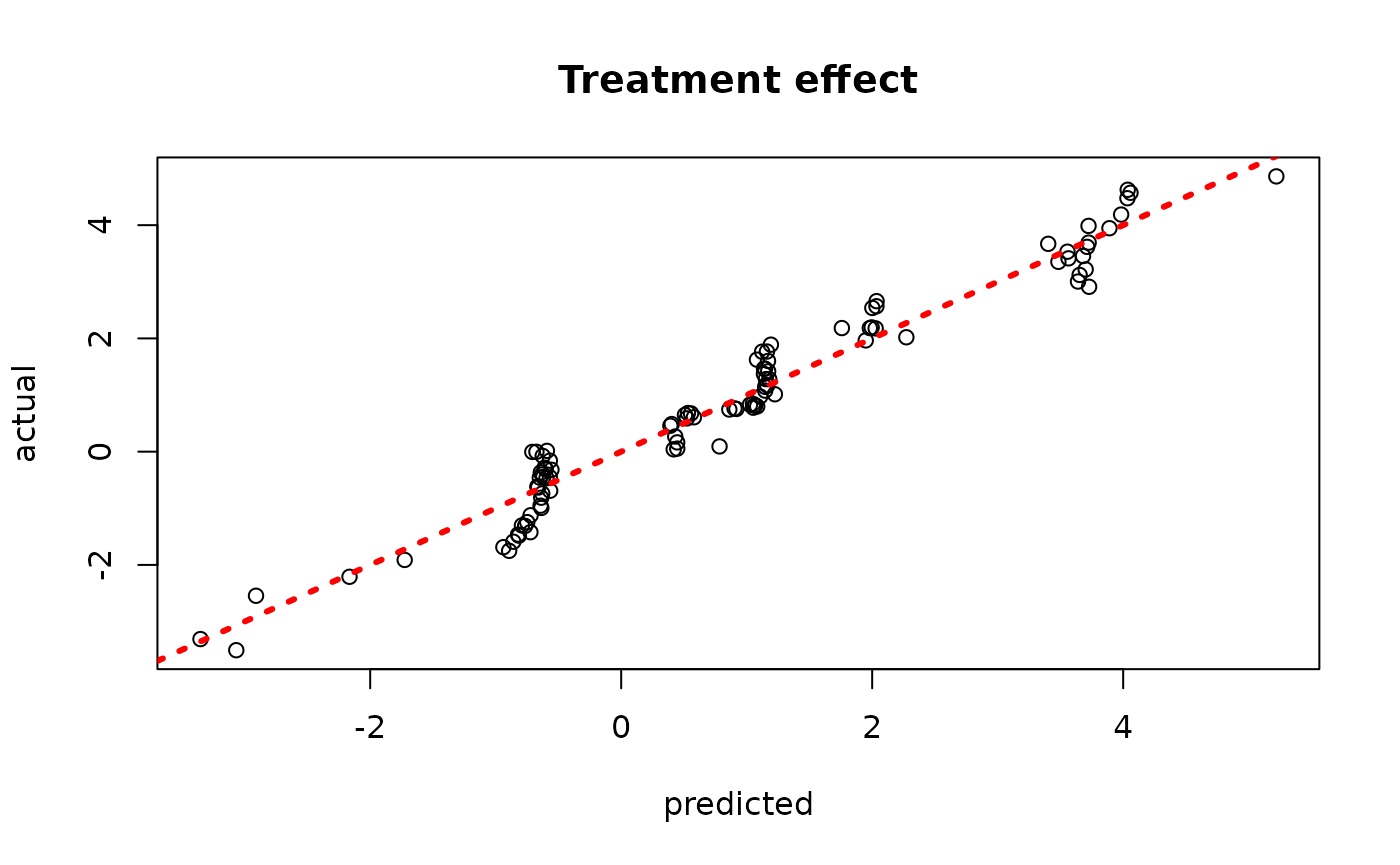
sigma_observed <- var(y-E_XZ)
plot_bounds <- c(min(c(bcf_model_root$sigma2_samples, sigma_observed)),
                 max(c(bcf_model_root$sigma2_samples, sigma_observed)))
plot(bcf_model_root$sigma2_samples, ylim = plot_bounds,
     ylab = "sigma^2", xlab = "Sample", main = "Global variance parameter")
abline(h = sigma_observed, lty=3, lwd = 3, col = "blue")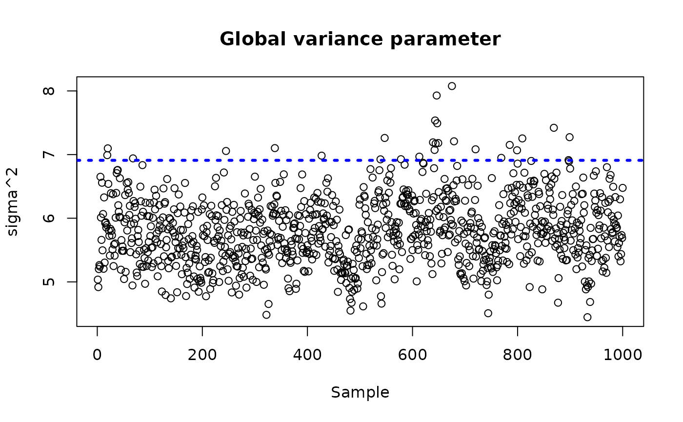
Examine test set interval coverage