Prior Calibration Approaches for Parametric Components of Stochastic Tree Ensembles

Background

The “classic” BART model of Chipman, George, and McCulloch (2010)

$$\begin{equation*} \begin{aligned} y &= f(X) + \epsilon\\ f(X) &\sim \text{BART}\left(\alpha, \beta\right)\\ \epsilon &\sim \mathcal{N}\left(0,\sigma^2\right)\\ \sigma^2 &\sim \text{IG}\left(a,b\right) \end{aligned} \end{equation*}$$

is semiparametric, with a nonparametric tree ensemble $f(X)$ and a homoskedastic error variance parameter $\sigma^2$. Note that in Chipman, George, and McCulloch (2010), $a$ and $b$ are parameterized with $a = \frac{\nu}{2}$ and $b = \frac{\nu\lambda}{2}$.

Setting Priors on Variance Parameters in stochtree

By default, stochtree employs a Jeffreys’ prior for $\sigma^2$$$\begin{equation*} \begin{aligned} \sigma^2 &\propto \frac{1}{\sigma^2} \end{aligned} \end{equation*}$$ which corresponds to an improper prior with $a = 0$ and $b = 0$.

We provide convenience functions for users wishing to set the $\sigma^2$ prior as in Chipman, George, and McCulloch (2010). In this case, $\nu$ is set by default to 3 and $\lambda$ is calibrated as follows:

1. An “overestimate,” $\hat{\sigma}^2$, of $\sigma^2$ is obtained via simple linear regression of $y$ on $X$
2. $\lambda$ is chosen to ensure that $p(\sigma^2 < \hat{\sigma}^2) = q$ for some value $q$, typically set to a default value of 0.9.

This is done in stochtree via the calibrate_inverse_gamma_error_variance function.

# Load library
library(stochtree)

# Generate data
n <- 1000
p <- 5
X <- matrix(runif(n*p), ncol = p)
f_XW <- (
    ((0 <= X[,1]) & (0.25 > X[,1])) * (-7.5) + 
    ((0.25 <= X[,1]) & (0.5 > X[,1])) * (-2.5) + 
    ((0.5 <= X[,1]) & (0.75 > X[,1])) * (2.5) + 
    ((0.75 <= X[,1]) & (1 > X[,1])) * (7.5)
)
noise_sd <- 1
y <- f_XW + rnorm(n, 0, noise_sd)

# Test/train split
test_set_pct <- 0.2
n_test <- round(test_set_pct*n)
n_train <- n - n_test
test_inds <- sort(sample(1:n, n_test, replace = FALSE))
train_inds <- (1:n)[!((1:n) %in% test_inds)]
X_test <- X[test_inds,]
X_train <- X[train_inds,]
y_test <- y[test_inds]
y_train <- y[train_inds]

# Calibrate the scale parameter for the variance term as in Chipman et al (2010)
nu <- 3
lambda <- calibrate_inverse_gamma_error_variance(y_train, X_train, nu = nu)

Now we run a BART model with this variance parameterization

bart_model <- bart(X_train = X_train, y_train = y_train, X_test = X_test, 
                   a_global = nu, b_global = nu*lambda, num_gfr = 0, 
                   num_burnin = 500, num_mcmc = 100)

Inspect the out-of-sample predictions of the model

plot(rowMeans(bart_model$y_hat_test), y_test, xlab = "predicted", ylab = "actual")
abline(0,1,col="red",lty=3,lwd=3)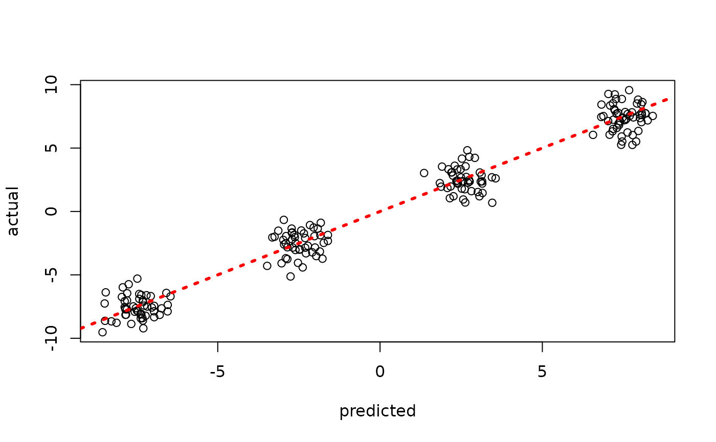

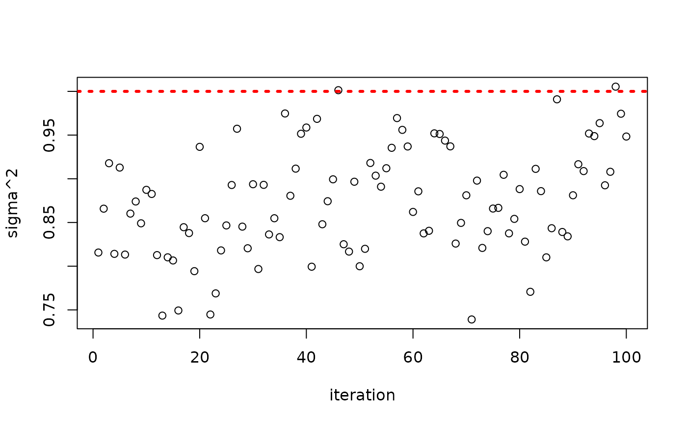
Inspect the posterior samples of $\sigma^2$

plot(bart_model$sigma2_samples, ylab = "sigma^2", xlab = "iteration")
abline(h = noise_sd^2, col = "red", lty = 3, lwd = 3)

References

Chipman, Hugh A., Edward I. George, and Robert E. McCulloch. 2010. “BART: Bayesian additive regression trees.” The Annals of Applied Statistics 4 (1): 266–98. https://doi.org/10.1214/09-AOAS285.